Symmetry-adapted basis sets
This page describes an advanced workflow: constructing a symmetry-adapted atomic-orbital basis (often called SALCs, symmetry-adapted linear combinations) and using it to transform matrices such as the overlap and Fock matrix into a block-diagonal form (one block per irreducible representation).
Why do this?
For molecules with non-trivial point-group symmetry, a symmetry-adapted basis can be used to:
reveal the symmetry structure of the AO space,
produce block-diagonal matrices (overlap, Fock, density),
reduce computational cost by working per symmetry block,
obtain orbitals that already carry irrep labels.
In PyQInt, the Hartree-Fock driver operates on atom-centered basis functions defined by the basis-set files. For advanced symmetry workflows, it is often useful to:
run a standard Hartree-Fock calculation to obtain matrices in the AO basis,
build a symmetry-adapted transformation matrix \(\mathbf{B}\),
transform matrices into the symmetry basis,
optionally reorder the symmetry basis to group irreps into consecutive blocks,
construct and visualize the resulting SALC basis functions.
Note
The example below focuses on (i) constructing SALCs and (ii) transforming matrices into a symmetry basis. A full SCF implementation in the symmetry basis (i.e. performing the SCF iterations per symmetry block) is a natural extension, but is not currently exposed as a separate high-level workflow.
Ethylene example
The script below demonstrates the construction of symmetry-adapted basis functions for ethylene, the transformation of the overlap matrix, and the visualization of the resulting SALCs.
import numpy as np

from pyqint import (
    MoleculeBuilder,
    HF,
    PyQInt,
    CGF,
    MatrixPlotter,
    ContourPlotter,
)

def main():
    # --------------------------------------------------------------------------
    # 1) Build the overlap matrix explicitly in the original AO basis
    # --------------------------------------------------------------------------
    mol = MoleculeBuilder.from_name("ethylene")
    cgfs, nuclei = mol.build_basis('sto3g')

    integrator = PyQInt()
    N = len(cgfs)
    S_ao = np.empty((N, N))

    for i in range(N):
        for j in range(i, N):
            S_ao[i, j] = S_ao[j, i] = integrator.overlap(cgfs[i], cgfs[j])

    # --------------------------------------------------------------------------
    # 2) Build an example symmetry-adaptation transformation B
    #    (This matrix is molecule- and AO-ordering-specific.)
    # --------------------------------------------------------------------------
    # Ethylene STO-3G yields 14 basis functions in this setup.
    B = np.zeros((14, 14))

    # Manally construct the SALCs (this is based on group theory)
    for i in range(0, 5):
        B[i * 2, i] = 1.0
        B[i * 2, i + 7] = 1.0
        B[i * 2 + 1, i] = 1.0
        B[i * 2 + 1, i + 7] = -1.0

    B[10, 5] = 1.0
    B[10, 6] = 1.0
    B[10, -2] = 1.0
    B[10, -1] = 1.0

    B[11, 5] = 1.0
    B[11, 6] = -1.0
    B[11, -2] = 1.0
    B[11, -1] = -1.0

    B[12, 5] = 1.0
    B[12, 6] = 1.0
    B[12, -2] = -1.0
    B[12, -1] = -1.0

    B[13, 5] = 1.0
    B[13, 6] = -1.0
    B[13, -2] = -1.0
    B[13, -1] = 1.0

    # --------------------------------------------------------------------------
    # 3) Transform the overlap matrix to the SALC basis:
    # --------------------------------------------------------------------------
    S_salc = B @ S_ao @ B.T

    # --------------------------------------------------------------------------
    # 4) Reorder SALCs so functions belonging to the same
    #    irreducible representation become consecutive,
    #    yielding block-diagonal matrices
    #
    #    A simple heuristic is used here: indices are grouped
    #    based on significant overlap matrix elements
    # --------------------------------------------------------------------------
    order = []
    for i in range(S_salc.shape[0]):
        for j in range(S_salc.shape[1]):
            if abs(S_salc[i, j]) > 0.1 and j not in order:
                order.append(j)

    P = np.zeros((len(order), len(order)), dtype=int)
    P[np.arange(len(order)), order] = 1
    B_blk = P @ B # construct block-diagonalized basis matrix

    # --------------------------------------------------------------------------
    # 5) Construct symmetry-adapted basis functions (SALCs)
    #    as new CGFs and perform a Hartree–Fock calculation
    #    directly in the SALC basis
    # --------------------------------------------------------------------------
    cgfs_salc = build_salcs_from_transform(cgfs, B_blk, integrator)
    res_salc = HF(mol, cgfs_salc).rhf(verbose=True)

    # --------------------------------------------------------------------------
    # 6) Define labels for symmetry blocks
    # --------------------------------------------------------------------------
    symfuncs = {
        r"A$_{g}$":  4,
        r"B$_{3u}$": 4,
        r"B$_{2g}$": 1,
        r"B$_{1u}$": 1,
        r"B$_{1g}$": 2,
        r"B$_{2u}$": 2,
    }

    symlabels = []
    for k, v in symfuncs.items():
        for i in range(v):
            symlabels.append(f"{k}({i+1})")

    # --------------------------------------------------------------------------
    # 7) Visualize block-structured matrices in the SALC basis
    # --------------------------------------------------------------------------
    # plot overlap matrix
    MatrixPlotter.plot_matrix(
        mat=res_salc['overlap'],
        filename="ethylene_overlap_salc.png",
        xlabels=symlabels,
        ylabels=symlabels,
        xlabelrot=90,
    )

    # plot fock matrix
    MatrixPlotter.plot_matrix(
        mat=res_salc['fock'],
        filename="ethylene_fock_salc.png",
        xlabels=symlabels,
        ylabels=symlabels,
        xlabelrot=90,
    )

    # plot coefficient matrix
    MatrixPlotter.plot_matrix(
        mat=res_salc['orbc'],
        filename="ethylene_coefficient_salc.png",
        xlabels=[r'$\psi_{%i}$' % (i+1) for i in range(len(res_salc['cgfs']))],
        ylabels=symlabels,
        xlabelrot=90,
    )

    # --------------------------------------------------------------------------
    # 8) Visualize symmetry-adapted basis functions (SALCs)
    #    as real-space contour plots
    # --------------------------------------------------------------------------
    # simple hack to visualize the basis functions
    res_salc['orbc'] = np.identity(res_salc['orbc'].shape[0])
    # custom defined planes
    planes = ['yz'] * res_salc['orbc'].shape[0]
    planes[8] = 'xy'
    planes[9] = 'xz'
    ContourPlotter.build_contourplot(
        res=res_salc,
        filename="ethylene_salcs_yz.png",
        plane=planes,
        sz=5.0,
        npts=101,
        nrows=2,
        ncols=7,
        labels=symlabels,
                    plot_energies = False,
    )

def build_salcs_from_transform(
    cgfs_ao,
    B: np.ndarray,
    integrator: PyQInt,
    threshold: float = 1e-2,
):
    """
    Construct SALC basis functions as CGFs using a linear transformation B.

    Each SALC is a linear combination of AO CGFs. Since the contributing AO
    primitives live on different atomic centers, primitives must be added
    with explicit positions using `add_gto_with_position`.

    The resulting SALCs are normalized individually.
    """
    n = B.shape[0]
    cgfs_salc = [CGF([0.0, 0.0, 0.0]) for _ in range(n)]

    for i in range(n):                 # new basis function index
        for j in range(len(cgfs_ao)):  # old AO basis function index
            w = float(B[i, j])
            if abs(w) < threshold:
                continue

            # Add all primitives of AO function j into SALC i
            for g in cgfs_ao[j].gtos:
                cgfs_salc[i].add_gto_with_position(
                    g.c * w,
                    g.p,
                    g.alpha,
                    g.l,
                    g.m,
                    g.n,
                )

        # Normalize SALC i: χ ← χ / sqrt(<χ|χ>)
        s_ii = integrator.overlap(cgfs_salc[i], cgfs_salc[i])
        norm = float(np.sqrt(s_ii))
        for g in cgfs_salc[i].gtos:
            g.c /= norm

    return cgfs_salc

if __name__ == "__main__":
    main()
Results for ethylene
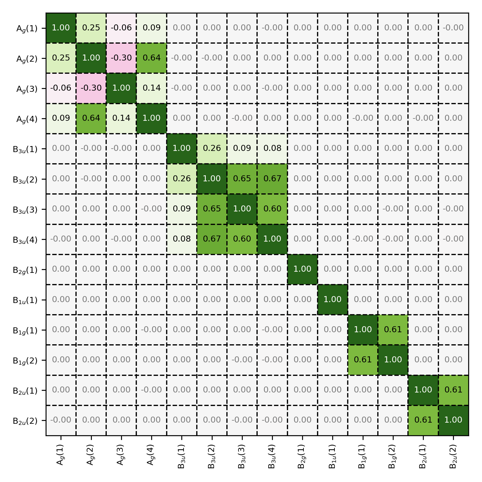
Overlap matrix in the symmetry-adapted basis. Observe that the overlap matrix has a block-diagonal structures, showing that the basis functions only overlap with other basis functions belonging to the same symmetry group.
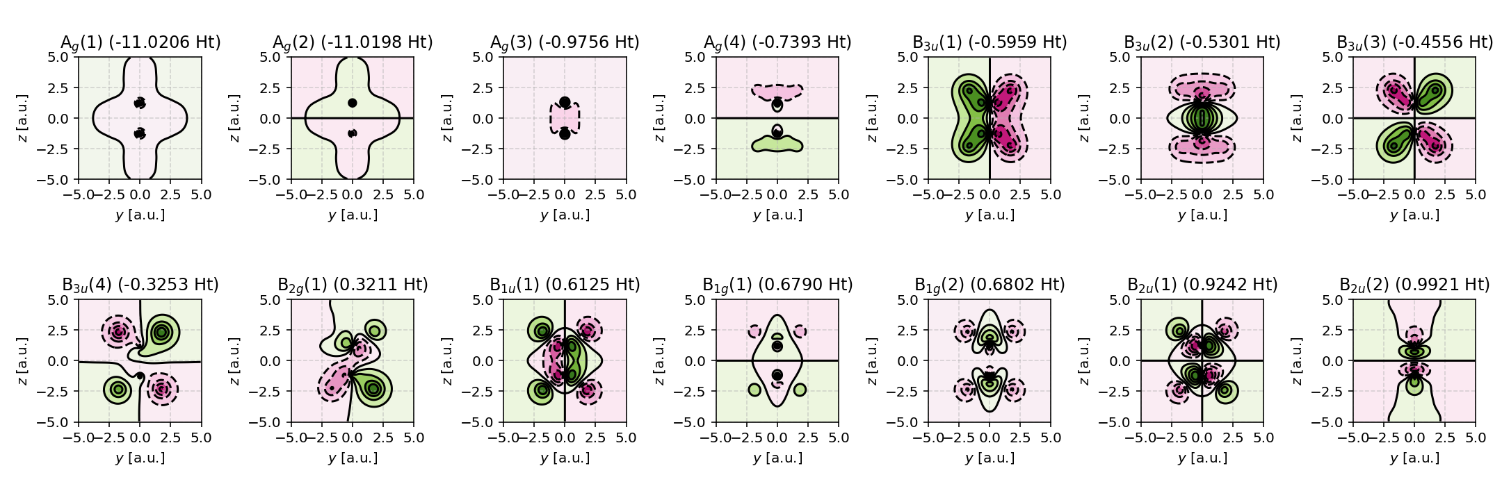
Contour plots of the symmetry adapted basis set. Note that the B3u and B2u basis functions constitute 2px orbitals are therefore cannot be visualized via a projection onto the \(yz\)-plane.
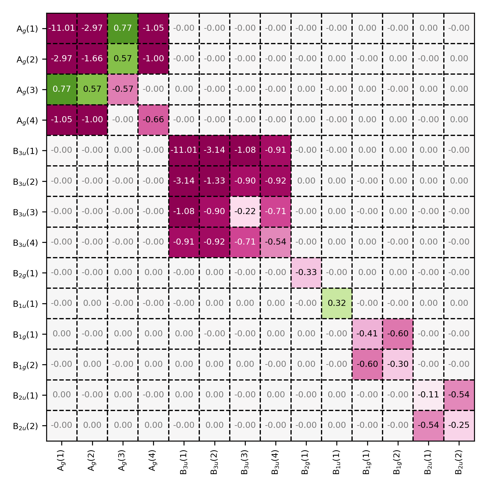
Fock matrix in the symmetry-adapted basis. Observe that the Fock matrix also has a block-diagonal structure.
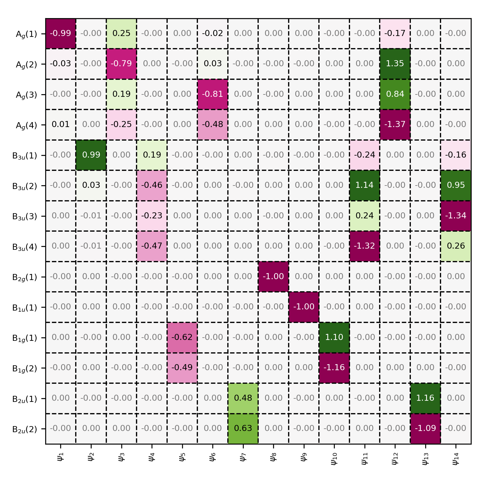
Coefficient matrix in the symmetry-adapted basis. All molecular orbitals are constructed from basis functions that belong to the same symmetry group.
Note
The transformation matrix \(\mathbf{B}\) is system- and ordering-dependent. In production workflows it is typically derived from the character table and projection operators for the molecule’s point group.
SALC construction requires combining primitives centered on different atoms. For this reason, the code uses
CGF.add_gto_with_positionwhen building the new contracted functions. During integral evaluation, the GTO centers are used, not the position stored in the CGF object itself.The reordering step uses a simple heuristic based on the transformed overlap matrix. For rigorous work, irrep assignment should be based on the explicit symmetry operations of the point group.