Orbital visualization

Since orbitals are essentially three-dimensional scalar fields, there are two useful procedures to visualize them. The scalar field can either be projected onto a plane, creating so-called contour plots. Alternatively, a specific value (i.e. the isovalue) of the scalar field can be chosen and all points in space that have this value can be tied together creating a so-called isosurface.

Contour plots can be easily created using matplotlib. For the creation of isosurfaces, we use PyTessel.

Contour plots

from pyqint import PyQInt, Molecule
import matplotlib.pyplot as plt
import numpy as np

# coefficients (calculated by Hartree-Fock using a sto3g basis set)
coeff = [8.37612e-17, -2.73592e-16,  -0.713011, -1.8627e-17, 9.53496e-17, -0.379323,  0.379323]

# construct integrator object
integrator = PyQInt()

# build water molecule
mol = Molecule('H2O')
mol.add_atom('O', 0.0, 0.0, 0.0)
mol.add_atom('H', 0.7570, 0.5860, 0.0)
mol.add_atom('H', -0.7570, 0.5860, 0.0)
cgfs, nuclei = mol.build_basis('sto3g')

# build grid
x = np.linspace(-2, 2, 50)
y = np.linspace(-2, 2, 50)
xx, yy = np.meshgrid(x,y)
zz = np.zeros(len(x) * len(y))
grid = np.vstack([xx.flatten(), yy.flatten(), zz]).reshape(3,-1).T
res = integrator.plot_wavefunction(grid, coeff, cgfs).reshape((len(y), len(x)))

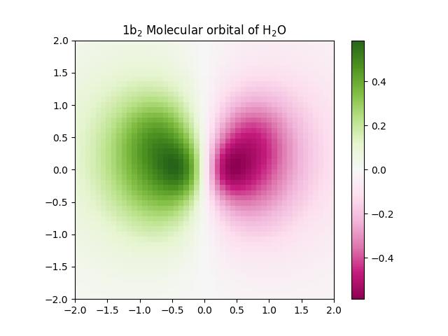
# plot wave function
plt.imshow(res, origin='lower', extent=[-2,2,-2,2], cmap='PiYG')
plt.colorbar()
plt.title('1b$_{2}$ Molecular orbital of H$_{2}$O')

ContourPlotter helper class

While contour plots can be constructed manually by explicitly building grids and evaluating molecular orbitals, PyQInt provides the ContourPlotter helper class to streamline this process.

The ContourPlotter class offers a single high-level interface for generating grids of contour plots for molecular orbitals obtained from a Hartree-Fock calculation. The class itself is intentionally stateless: all required information is passed explicitly via the Hartree-Fock results object.

Warning

ContourPlotter methods currently only support restricted Hartree-Fock calculations.

Cartesian-aligned contour plots

The simplest usage corresponds to contour plots aligned with one of the Cartesian coordinate planes (\(xy\), \(xz\), or \(yz\)). The plane is specified using a string identifier.

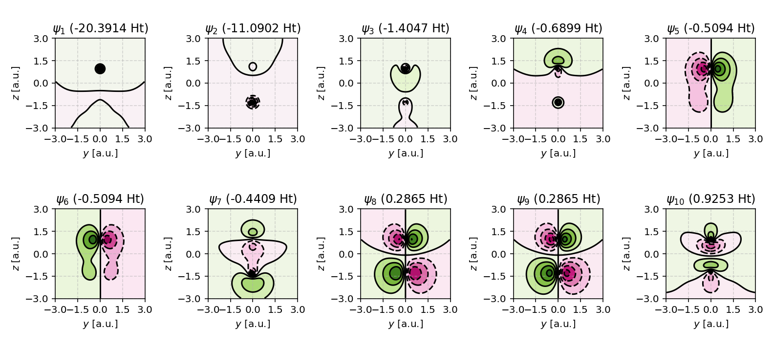
The following example visualizes the molecular orbitals of carbon monoxide (CO) in the \(yz\) plane:

from pyqint import MoleculeBuilder, HF, ContourPlotter

mol = MoleculeBuilder.from_name('CO')
res = HF(mol, 'sto3g').rhf(verbose=True)

ContourPlotter.build_contourplot(
    res,
    'co_contour.png',
    plane='yz',
    sz=3.0,
    npts=101,
    nrows=2,
    ncols=5
)

In this example, the contour plots are centered at the origin, span a square region of width \(2 \times \text{sz}\), and display the lowest ten molecular orbitals in a \(2 \times 5\) grid.

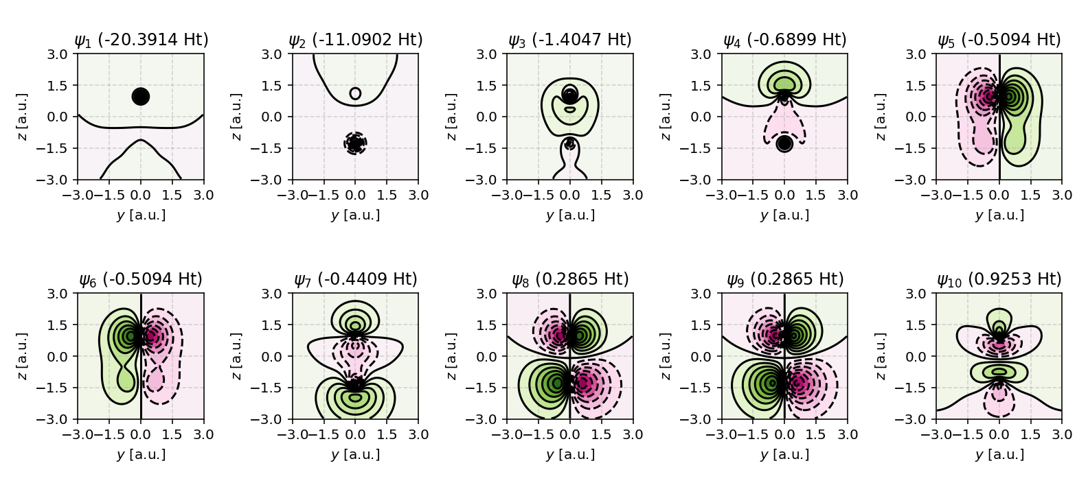
Tip

Want more contour levels? Simply adjust the levels argument.

ContourPlotter.build_contourplot(
    res,
    'co_contour_level15.png',
    plane='yz',
    sz=3.0,
    npts=101,
    nrows=2,
    ncols=5,
    levels=15 # adjust this value
)

Arbitrary planar contour plots

In many situations, it is desirable to visualize molecular orbitals in planes that are not aligned with the Cartesian axes. Typical examples include planes defined by three atoms or planes aligned with molecular symmetry elements. The ContourPlotter supports such cases by allowing the plane to be defined using three atoms and an explicit up direction. The three atoms uniquely define the plane, while the up direction removes the sign ambiguity of the plane normal.

The plane specification is given as a tuple:

\[(i, j, k, \vec{u})\]

where:

• \(i\), \(j\), and \(k\) are atom indices defining the plane

• \(\vec{u}\) is a reference vector that orients the plane normal

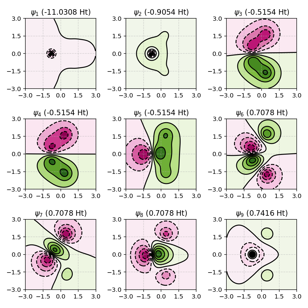
The following example visualizes molecular orbitals of methane (CH₄) in a plane defined by three hydrogen atoms, with the \(z\) axis chosen as the up direction:

from pyqint import MoleculeBuilder, HF, ContourPlotter

mol = MoleculeBuilder.from_name('CH4')
res = HF(mol, 'sto3g').rhf(verbose=True)

up = [0, 0, 1]
ContourPlotter.build_contourplot(
    res,
    'ch4_contour.png',
    plane=(0, 1, 2, up), # note: this needs to be a tuple
    sz=3.0,
    npts=101,
    nrows=3,
    ncols=3
)

In this case, the plotting plane is constructed as follows:

1. The three selected atoms define a geometric plane.

2. The plane normal is computed from the atomic positions.

3. The normal is oriented consistently with the supplied up direction.

4. A local orthonormal coordinate system is constructed within the plane.

5. A two-dimensional grid is embedded into three-dimensional space.

This approach makes it possible to visualize molecular orbitals in any chemically meaningful plane, independent of the global coordinate system.

Constructing isosurfaces

Note

• Isosurface generation requires the PyTessel package to be installed. Make sure you have installed PyTessel alongside PyQInt. For more details, see the Installation.

• Optionally, have a look at PyTessel’s documentation.

from pyqint import PyQInt, Molecule, HF
import numpy as np
from pytessel import PyTessel

def main():
    # calculate sto3g coefficients for h2o
    cgfs, coeff = calculate_co()

    # build isosurface of the fifth MO
    # isovalue = 0.1
    # store result as .ply file
    build_isosurface('co_04.ply', cgfs, coeff[:,4], 0.1)

def build_isosurface(filename, cgfs, coeff, isovalue):
    # generate some data
    sz = 100
    integrator = PyQInt()
    grid = integrator.build_rectgrid3d(-5, 5, sz)
    scalarfield = np.reshape(integrator.plot_wavefunction(grid, coeff, cgfs), (sz, sz, sz))
    unitcell = np.diag(np.ones(3) * 10.0)

    pytessel = PyTessel()
    vertices, normals, indices = pytessel.marching_cubes(scalarfield.flatten(), scalarfield.shape, unitcell.flatten(), isovalue)
    pytessel.write_ply(filename, vertices, normals, indices)

def calculate_co():
    mol = Molecule()
    mol.add_atom('C', 0.0, -0.5, 0.0)
    mol.add_atom('O', 0.0, 0.5, 0.0)

    result = HF(mol, 'sto3g').rhf()

    return result['cgfs'], result['orbc']

if __name__ == '__main__':
    main()

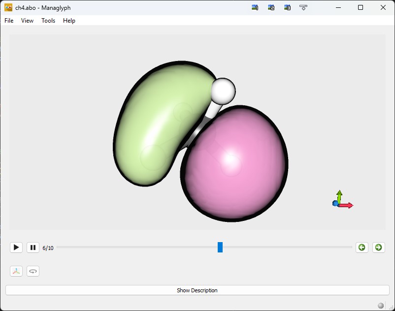
Constructing ABO files

PyQInt can be interfaced with ABO Builder to generate .abo files that can be visualized using Managlyph. Managlyph enables straightforward rendering of molecular orbitals and interactive 3D visualization, including stereoscopic viewing with red/cyan glasses.

First, install ABO Builder:

pip install abobuilder

The script below demonstrates how to generate an .abo file directly from a Hartree-Fock calculation. For best performance, it is recommended to use the build_abo_hf_v1 function with compression enabled.

If the molecular orbitals appear too coarse, increase the nsamples parameter to improve grid resolution. If orbitals appear spatially truncated, increase the sampling box size using the sz parameter.

import os

from abobuilder import AboBuilder, clean_multiline
from pyqint import MoleculeBuilder, HF

# Build the molecule and perform a Hartree–Fock calculation
ch4 = MoleculeBuilder().from_name('CH4')
res = HF(ch4, basis='sto3g').rhf(verbose=True)

# Geometry frame description
desc = clean_multiline(
    """
    Canonical molecular orbitals for CH4 (STO-3G), computed with PyQInt.
    Generated with ABO Builder.
    """
)

# Create the ABOF v1 file with compression enabled
if not os.path.exists('ch4.abo'):
    AboBuilder().build_abo_hf_v1(
        'ch4.abo',
        res['nuclei'],
        res['cgfs'],
        res['orbc'],
        res['orbe'],
        nsamples=51,
        compress=True,
        geometry_descriptor=desc,
    )

The resulting file (ch4.abo) should be around 865 kb in size. This file can be readily opened using Managlyph. Below, a representative screenshot is provided.