Orbital localization: Foster-Boys

Warning

Orbital Localization methods currently only support restricted Hartree-Fock calculations.

Background of FB

The canonical orbitals of a Hartree-Fock calculation are defined such that these will diagonalize the Fock-matrix by which these molecular orbitals are eigenfunctions of the Fock-operator. Nevertheless, this set of solutions is not unique in the sense that multiple sets of molecular orbitals produce the same electron density and the same total electronic energy. One is allowed to perform an arbitrary unitary transformations on the set of occupied orbitals yielding a new set that is as good as a representation as the old set. Some of these representations are however more useful than others and one particular useful representation is the one that makes the orbitals as localized (compact and condensed) as possible.

The degree of localization can be captured via relatively simple metric as given by

\[\mathcal{M} = \sum_{i \in \textrm{occ}} \left<\psi_{i} | \vec{r} | \psi_{i} \right>^{2}\]

where \(\psi_{i}\) is a molecular orbital and \(i\) loops over the occupied molecular orbitals. One obtains (perhaps counter-intuitively) the most localized orbitals by maximizing the value of mathcal{M}.

The process of mixing the molecular orbitals among themselves to the aim of maximizing is mathcal{M} is embedded in the FosterBoys class.

Procedure of FB

The code below first performs a Hartree-Fock calculation on the CO molecule after which the localized molecular orbitals are calculated using the Foster-Boys method. The Foster-Boys localization procedure is present as a separate class in the PyQInt package. It takes the output of a Hartree-Fock calculation as its input.

Note

The code below uses the PyTessel package for constructing the isosurfaces. PyTessel is an external package for easy construction of isosurfaces from scalar fields. More information is given in the corresponding section.

from pyqint import Molecule, HF, PyQInt, FosterBoys
import pyqint
import numpy as np
from pytessel import PyTessel

def main():
    res = calculate_co(1.145414)
    resfb = FosterBoys(res).run()

    for i in range(len(res['cgfs'])):
        build_isosurface('MO_%03i' % (i+1),
                         res['cgfs'],
                         resfb['orbc'][:,i],
                         0.1)

def calculate_co(d):
    """
    Full function for evaluation
    """
    mol = Molecule()
    mol.add_atom('C', 0.0, 0.0, -d/2, unit='angstrom')
    mol.add_atom('O', 0.0, 0.0,  d/2, unit='angstrom')

    result = HF(mol, 'sto3g').rhf()

    return result

def build_isosurface(filename, cgfs, coeff, isovalue, sz=5, npts=100):
    # generate some data
    isovalue = np.abs(isovalue)
    integrator = PyQInt()
    grid = integrator.build_rectgrid3d(-sz, sz, npts)
    scalarfield = np.reshape(integrator.plot_wavefunction(grid, coeff, cgfs), (npts, npts, npts))
    unitcell = np.diag(np.ones(3) * 2 * sz)

    pytessel = PyTessel()
    vertices, normals, indices = pytessel.marching_cubes(scalarfield.flatten(), scalarfield.shape, unitcell.flatten(), isovalue)
    fname = filename + '_pos.ply'
    pytessel.write_ply(fname, vertices, normals, indices)

    vertices, normals, indices = pytessel.marching_cubes(scalarfield.flatten(), scalarfield.shape, unitcell.flatten(), -isovalue)
    fname = filename + '_neg.ply'
    pytessel.write_ply(fname, vertices, normals, indices)

if __name__ == '__main__':
    main()

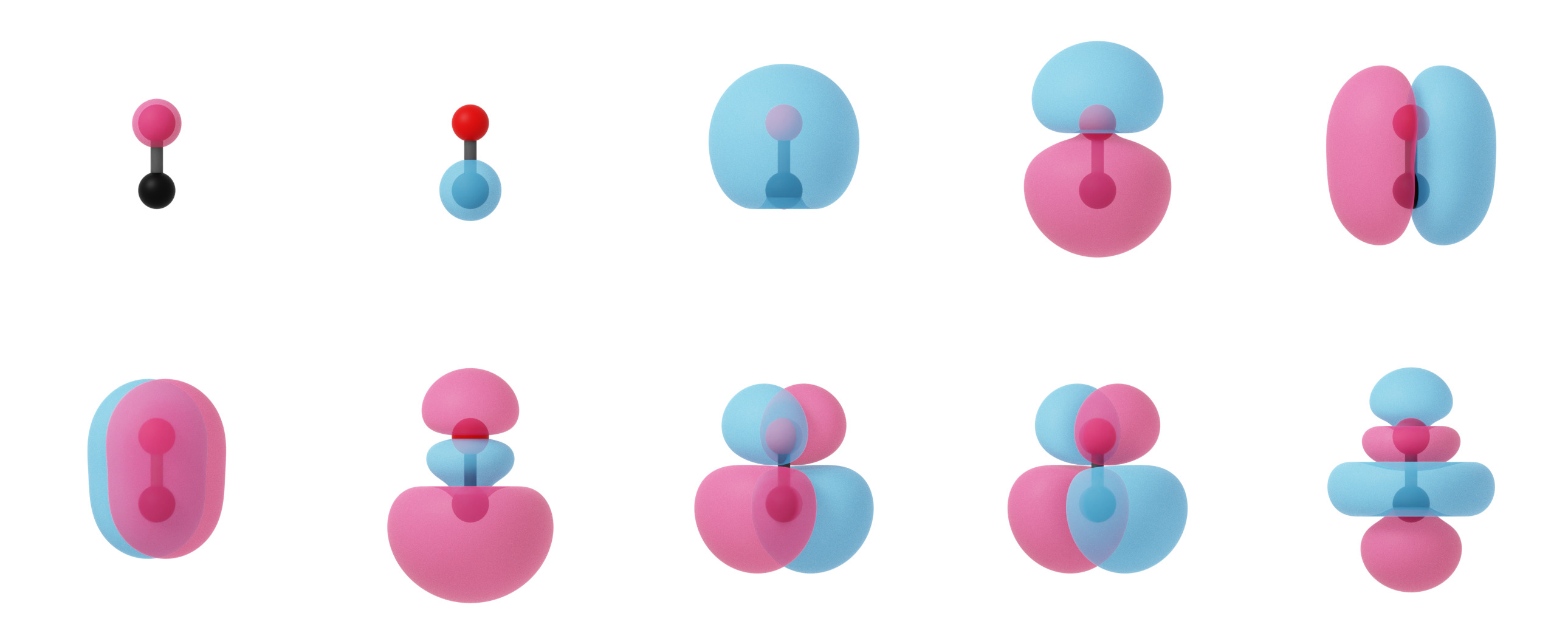
Canonical molecular orbitals of CO visualized using isosurfaces with an isovalue of +/-0.03.

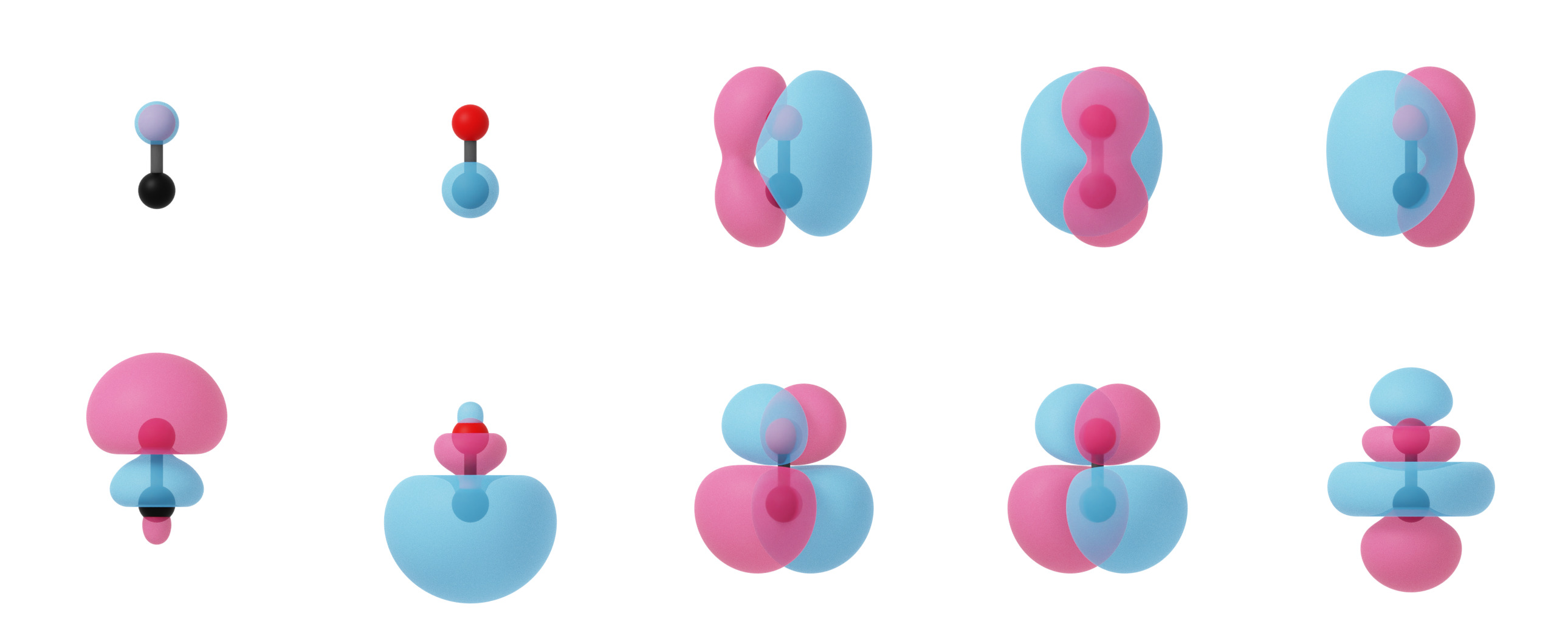
Localized molecular orbitals of CO visualized using isosurfaces with an isovalue of +/-0.03. Note that the localization procedure has only been applied to the occupied molecular orbitals. Observe that the localized orbitals contain a triple-degenerate state corresponding to the triple bond and two lone pairs for C and O.

Foster-Boys output object

The output object of a Foster-Boys calculation is very similar to the one of a Hartree-Fock calculation. It is a dictionary that contains the following elements.

Description of the data contained in the result library

Key	Description
orbe	Orbital energies after the unitary transformation.
orbc	Orbital coefficient after the unitary transformation.
nriter	Number of iterations.
r2start	Initial sum of the squared dipole moment norm of the molecular orbitals.
r2final	Final sum of the squared dipole moment norm of the molecular orbitals.

Hint

One can directly connect the output of a Foster-Boys calculation to a COHP calculation. The details of the process are found in the cohp analysis of Foster-Boys localized orbitals section.