Geometry optimization
Performing a geometry optimization
PyQInt is able to perform a geometry optimization of a molecule. It
should however be noted that this functionality is rather limited and essentially
makes use of existing routines available in Scipy,
specifically the scipy.optimize.minimize routine using the
conjugate gradient method.
To demonstrate the procedure, let us consider the CH4 molecule in a non-converged geometry wherein the C-H bonds are longer than their optimal value and where the C molecule does not lie in the middle of the 4 hydrogen atoms.
Geometry optimization is handled by the GeometryOptimization class
which takes a molecule and a basis set as input. The user can indicate whether
they prefer verbose output or not. By default, geometry optimization is silent
and does not yield any output.
from pyqint import GeometryOptimization, Molecule

mol = Molecule()
dist = 1.0
mol.add_atom('C', 0.1, 0.0, 0.1, unit='angstrom')
mol.add_atom('H', dist, dist, dist, unit='angstrom')
mol.add_atom('H', -dist, -dist, dist, unit='angstrom')
mol.add_atom('H', -dist, dist, -dist, unit='angstrom')
mol.add_atom('H', dist, -dist, -dist, unit='angstrom')

res = GeometryOptimization(mol, 'sto3g', verbose=True).run()
The output of the above script (condensed) is:
################################################################################
START GEOMETRY OPTIMIZATION (CONJUGATE GRADIENT)
################################################################################

================================================================================
GEOMETRY OPTIMIZATION STEP 001
================================================================================

--------------------------------------------------------------------------------
    ENERGIES
--------------------------------------------------------------------------------

Kinetic:                      39.25313761
Nuclear:                     -108.88180088
Electron-electron repulsion:  28.15082009
Exchange:                     -6.09926245
Nuclear repulsion:             8.45508042
TOTAL:                       -39.12202512

--------------------------------------------------------------------------------
    POSITIONS AND FORCES
--------------------------------------------------------------------------------

C  |   0.100000   0.000000   0.100000 | +1.6500e-02 +2.2923e-04 +1.6500e-02
H  |   1.000000   1.000000   1.000000 | +4.3454e-02 +5.0855e-02 +4.3454e-02
H  |  -1.000000  -1.000000   1.000000 | -5.2300e-02 -4.5705e-02 +3.8773e-02
H  |  -1.000000   1.000000  -1.000000 | -4.6427e-02 +4.0325e-02 -4.6427e-02
H  |   1.000000  -1.000000  -1.000000 | +3.8773e-02 -4.5705e-02 -5.2300e-02

Elapsed time: 0.2787 s

================================================================================

================================================================================
GEOMETRY OPTIMIZATION STEP 002
================================================================================

--------------------------------------------------------------------------------
    ENERGIES
--------------------------------------------------------------------------------

Kinetic:                      39.15432005
Nuclear:                     -109.64153523
Electron-electron repulsion:  28.55699241
Exchange:                     -6.14351258
Nuclear repulsion:             8.85933154
TOTAL:                       -39.21440452

--------------------------------------------------------------------------------
    POSITIONS AND FORCES
--------------------------------------------------------------------------------

C  |   0.083500  -0.000229   0.083500 | +1.5463e-02 +6.8533e-04 +1.5463e-02
H  |   0.956546   0.949145   0.956546 | +4.4324e-02 +5.0368e-02 +4.4324e-02
H  |  -0.947700  -0.954295   0.961227 | -5.2664e-02 -4.7060e-02 +4.1251e-02
H  |  -0.953573   0.959675  -0.953573 | -4.8374e-02 +4.3066e-02 -4.8374e-02
H  |   0.961227  -0.954295  -0.947700 | +4.1251e-02 -4.7060e-02 -5.2664e-02

Elapsed time: 0.2461 s

================================================================================

...

================================================================================
GEOMETRY OPTIMIZATION STEP 033
================================================================================

--------------------------------------------------------------------------------
    ENERGIES
--------------------------------------------------------------------------------

Kinetic:                      39.46555789
Nuclear:                     -118.95694319
Electron-electron repulsion:  32.86550181
Exchange:                     -6.62307658
Nuclear repulsion:            13.52209655
TOTAL:                       -39.72686316

--------------------------------------------------------------------------------
    POSITIONS AND FORCES
--------------------------------------------------------------------------------

C  |   0.019995   0.000002   0.019995 | +3.4887e-06 +2.7088e-06 +3.4885e-06
H  |   0.645172   0.625454   0.645172 | -3.0848e-06 -5.6713e-06 -3.0848e-06
H  |  -0.605171  -0.625272   0.645388 | +4.1945e-07 -6.8789e-08 +2.2218e-06
H  |  -0.605385   0.625087  -0.605385 | -3.0450e-06 +3.1000e-06 -3.0450e-06
H  |   0.645388  -0.625272  -0.605171 | +2.2217e-06 -6.8771e-08 +4.1955e-07

Elapsed time: 0.2467 s

================================================================================

================================================================================
GEOMETRY OPTIMIZATION STEP 034
================================================================================

--------------------------------------------------------------------------------
    ENERGIES
--------------------------------------------------------------------------------

Kinetic:                      39.46555331
Nuclear:                     -118.95690650
Electron-electron repulsion:  32.86548664
Exchange:                     -6.62307497
Nuclear repulsion:            13.52207800
TOTAL:                       -39.72686370

--------------------------------------------------------------------------------
    POSITIONS AND FORCES
--------------------------------------------------------------------------------

C  |   0.019993   0.000002   0.019993 | +1.1853e-06 +1.5988e-06 +1.1850e-06
H  |   0.645174   0.625454   0.645174 | -1.6340e-06 -4.6101e-06 -1.6340e-06
H  |  -0.605170  -0.625272   0.645390 | +5.5012e-07 -1.2756e-07 +2.7956e-06
H  |  -0.605386   0.625089  -0.605386 | -2.8970e-06 +3.2663e-06 -2.8970e-06
H  |   0.645390  -0.625272  -0.605170 | +2.7956e-06 -1.2747e-07 +5.5023e-07

Elapsed time: 0.2813 s

================================================================================
Result dictionary of a geometry optimization
The result of a Geometry Optimization calculation is captured inside a dictionary object. This dictionary objects contains the following keys
Key |
Description |
|---|---|
|
|
|
List of the total electronic energy at each ionic step. |
|
List of the forces on all the atoms at each ionic step. |
|
Coordinates of the atoms at each ionic step. |
|
Result dictionary of the Hartree-Fock calculation last ionic step. |
|
Molecule on which the geometry optimization acted. |
To demonstrate the use of the above data, consider the script as shown below.
In this script, we generate a CH4 in a (highly) perturbed configuration.
The perturbed configuration is generated using a random number generator (RNG). For
reproduction purposes, we have seeded this RNG such that the result as shown
below can be easily reproduced. The result of the geometry optimization is
captured in the res variable which is a dictionary according to the
above-mentioned specifications.
To show how the contents of this dictionary can be used, we produce two plots which are explained below.
from pyqint import GeometryOptimization, Molecule
import matplotlib.pyplot as plt
import numpy as np

# seed the random number generator to yield reproducible result
np.random.seed(4)

# build a CH4 molecule where the atom positions are perturbed based on a
# random number generator
mol = Molecule()
dist = 1.0
mol.add_atom('C', 0.1, 0.0, 0.1, unit='angstrom')
mol.add_atom('H', dist + np.random.rand(),
                  dist + np.random.rand(),
                  dist + np.random.rand(),
                  unit='angstrom')
mol.add_atom('H', -dist + np.random.rand(),
                  -dist + np.random.rand(),
                  dist + np.random.rand(),
                  unit='angstrom')
mol.add_atom('H', -dist + np.random.rand(),
                  dist + np.random.rand(),
                  -dist + np.random.rand(),
                  unit='angstrom')
mol.add_atom('H', dist + np.random.rand(),
                  -dist + np.random.rand(),
                  -dist + np.random.rand(),
                  unit='angstrom')

# perform the geometry optimization
res = GeometryOptimization(verbose=False).run(mol, 'sto3g')

# collect the RMS of the force
rms = np.zeros(len(res['coordinates']))
for i in range(len(res['coordinates'])):
    forces = res['forces'][i]
    rms[i] = np.sqrt(np.sum(np.linalg.norm(forces, axis=0) / float(len(forces))))

# plot electronic energy and RMS of the force
fig, ax1 = plt.subplots(dpi=144, figsize=(6,4))
ax1.plot(res['energies'], '-o', color='black')
ax2 = plt.twinx()
ax2.plot(rms, '-o', color='red')
ax2.set_ylabel('Root-mean-square force')
ax2.tick_params(axis='y', colors='red')
ax2.yaxis.label.set_color('red')
ax2.spines['right'].set_color('red')
ax1.grid(linestyle='--', color='black', alpha=0.5)
ax1.set_xlabel('Iteration [-]')
ax1.set_ylabel('Electronic energy [Ht]')
plt.tight_layout()
plt.show()

# show convergence of C-H bond distances for all bonds
# collect data
distances = np.zeros((4, len(res['coordinates'])))
for i in range(0,4):
    for j in range(0, len(res['coordinates'])):
        coord = res['coordinates'][j]
        distances[i,j] = np.linalg.norm(coord[i+1] - coord[0])

# plot in a figure
plt.figure(dpi=144, figsize=(6,4))
for i in range(0,4):
    plt.plot(distances[i,:], '-o', alpha=0.5, label='H$_{%i}$' % (i+1))
plt.grid(linestyle='--', color='black', alpha=0.5)
plt.xlabel('Iteration [-]')
plt.ylabel('C-H bond distance [Bohr]')
plt.legend(loc='right')
plt.tight_layout()
plt.show()
The result of the above script are the following two images, showcasing the optimization procedure and an example application of the data in the result dictionary. The first figure shows the total electronic energy and the root-mean-square of the force as function of the iteration number. The convergence criterion is essentially such that these forces need to be smaller than a threshold value. From the figure, it is clear that the total electronic energy converges faster than the forces.
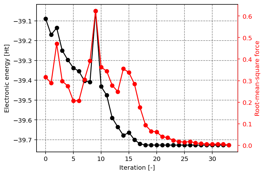
Energy and root-mean-square of the forces as function of the iteration number.
In the second figure, we can observe the C-H bond distance as function of the iteration number. Clearly, we start at a relatively unfavorable geometry where one of the H atoms is quite distanced from the central C atom. With increasing iteration, we can however readily see that all C-H bond distances converge to the same value, as expected for the highly symmetric CH4 molecule.
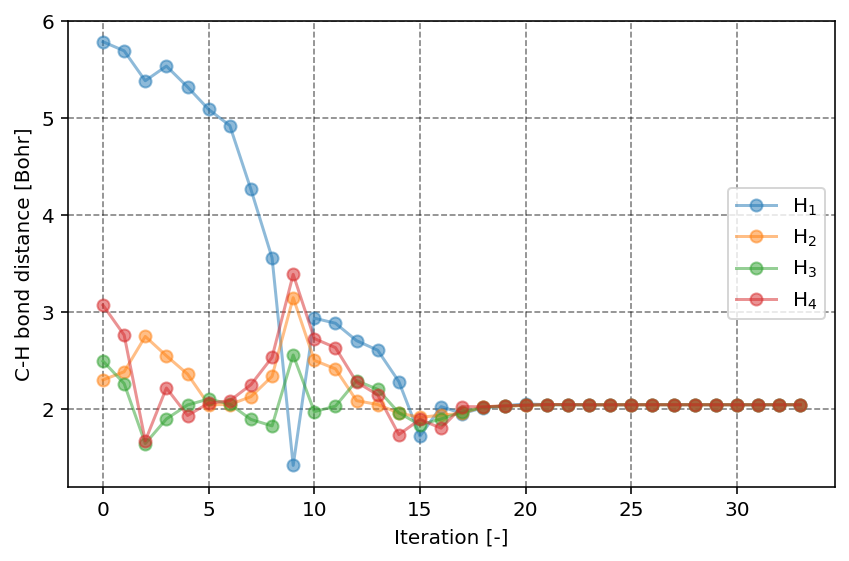
C-H bond distances as function of the iteration number.
Danger
It is by no means guaranteed that a geometry optimization converges. Even more important, when the geometry optimization has not converged, it is also highly likely that the underlying electronic structure calculation has not been properly converged as well. One should absolutely distrust any result coming out of such a calculation.
Always verify that a calculation is properly converged before using its output.