Matrix visualization
Many quantities encountered in electronic-structure theory are naturally
represented as matrices, such as overlap matrices, Fock matrices, or molecular
orbital coefficient matrices. To facilitate the inspection and interpretation
of such data, PyQInt provides the MatrixPlotter helper class.
The MatrixPlotter is intentionally stateless and offers a compact
interface for visualizing square matrices as annotated heatmaps. Each matrix
element is displayed both by color and by its numerical value, making the
structure and magnitude of matrix elements immediately apparent.
Atomic orbital labeling
For chemically meaningful matrix plots, it is often desirable to label rows and
columns using atomic orbital (AO) labels. Since AO labels cannot be inferred
unambiguously from contracted Gaussian functions alone, the
MatrixPlotter provides a helper routine (generate_ao_labels) for
generating AO labels from an explicit shell specification.
AO labels are generated by providing for each atom its element symbol and the list of shells that should be included. The shell specification explicitly defines the principal quantum number and angular momentum and avoids any ambiguity associated with multiple shells of identical angular momentum.
# example to generate AO labels for CO
labels = MatrixPlotter.generate_ao_labels([
    ('O', ('1s', '2s', '2p')),
    ('C', ('1s', '2s', '2p')),
])
Example: overlap, Fock, and coefficient matrices of CO
The following example demonstrates how to visualize the overlap matrix, Fock matrix, and molecular orbital coefficient matrix of carbon monoxide (CO) computed at the Hartree–Fock/STO-3G level.
from pyqint import MoleculeBuilder, HF, MatrixPlotter

def main():
    mol = MoleculeBuilder().from_name('CO')
    res = HF(mol, 'sto3g').rhf(verbose=False)

    labels = MatrixPlotter.generate_ao_labels([
        ('O', ('1s', '2s', '2p')),
        ('C', ('1s', '2s', '2p')),
    ])

    MatrixPlotter.plot_matrix(
        mat=res['overlap'],
        filename='overlap-co.png',
        xlabels=labels,
        ylabels=labels,
        xlabelrot=0,
        title='Overlap',
    )

    MatrixPlotter.plot_matrix(
        mat=res['fock'],
        filename='fock-co.png',
        xlabels=labels,
        ylabels=labels,
        xlabelrot=0,
        title='Fock',
    )

    MatrixPlotter.plot_matrix(
        mat=res['orbc'],
        filename='coefficient-co.png',
        xlabels=[r'$\psi_{%i}$' % (i+1) for i in range(len(res['cgfs']))],
        ylabels=labels,
        xlabelrot=0,
        title='Coefficient',
    )

if __name__ == '__main__':
    main()
In this example:
The overlap and Fock matrices are visualized using AO labels on both axes.
The molecular orbital coefficient matrix is visualized with atomic orbitals along the rows and molecular orbitals along the columns.
The figure size is determined automatically from the matrix dimension, while the output filename is specified explicitly for each plot.
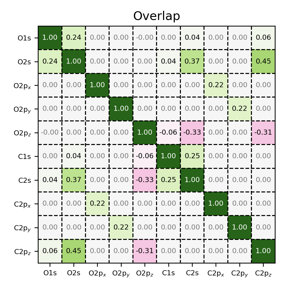
Overlap matrix of CO, visualized using the MatrixPlotter class.
Note that the entries on the diagonal are all equal to one, indicating
that the basis set is normalized. Also note that because of the symmetry
of the molecule, certain elements of the matrix are equal to zero.
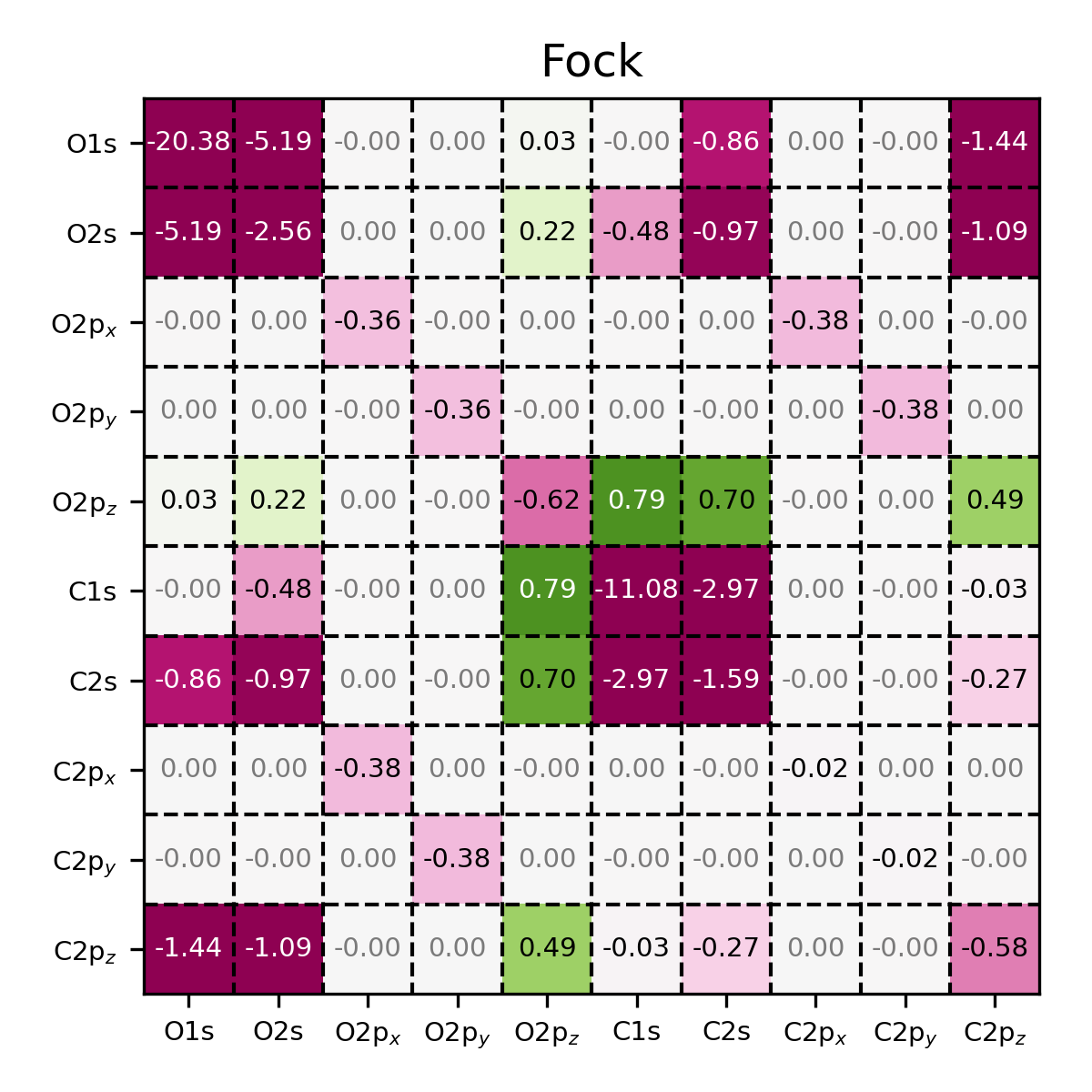
Fock matrix of CO, visualized using the MatrixPlotter class. Observe
that the first and sixth diagonal element have significantly lower energies,
indicating that these basis functions correspond to core atomic orbitals.
Also note that because of the symmetry of the molecule, certain elements
of the matrix are equal to zero, similar to the overlap matrix.
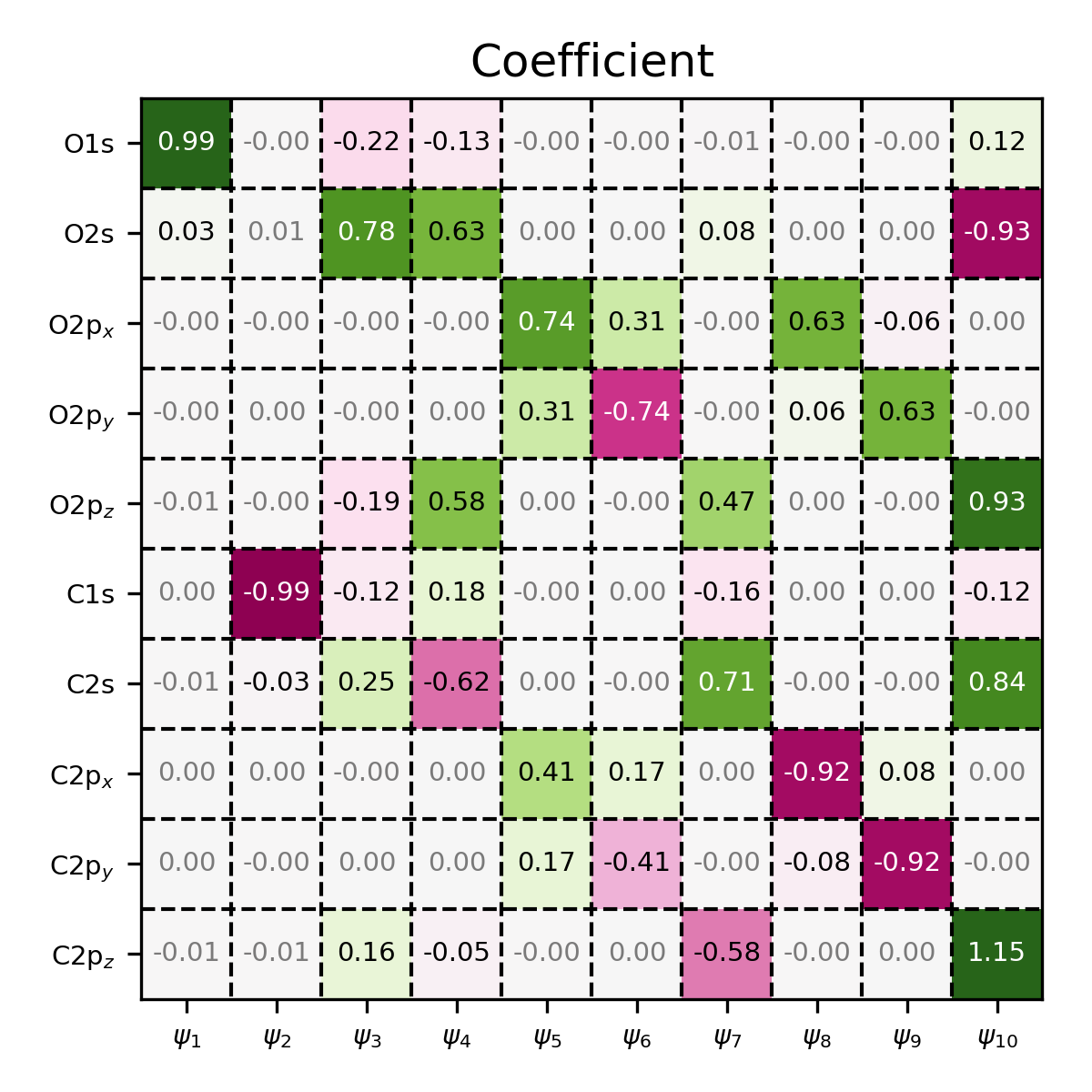
Coefficient matrix of CO, visualized using the MatrixPlotter class.
Highlighting elements
In some cases, it is useful not only to visualize a matrix, but also to
emphasize specific elements or regions within it. This can be achieved using
the boxes argument.
The boxes argument expects a list of 5-tuples. Each tuple defines a
rectangular region and consists of the following elements, in order:
the starting x-coordinate
the starting y-coordinate
the width of the rectangle
the height of the rectangle
the color of the rectangle
The example below demonstrates how to draw red, green, and blue rectangles on top of a matrix visualization.
from pyqint import MoleculeBuilder, HF, MatrixPlotter

def main():
    mol = MoleculeBuilder().from_name('CO')
    res = HF(mol, 'sto3g').rhf(verbose=False)

    labels = MatrixPlotter.generate_ao_labels([
        ('O', ('1s', '2s', '2p')),
        ('C', ('1s', '2s', '2p')),
    ])

    # highlighting boxes
    boxes = [
        (0,0,1,1,'#BB0000'),
        (1,2,3,1,'#00BB00'),
        (3,4,1,3,'#0000BB'),
    ]

    MatrixPlotter.plot_matrix(
        mat=res['overlap'],
        filename='overlap-co.png',
        xlabels=labels,
        ylabels=labels,
        xlabelrot=0,
        title='Overlap',
        boxes=boxes
    )

if __name__ == '__main__':
    main()
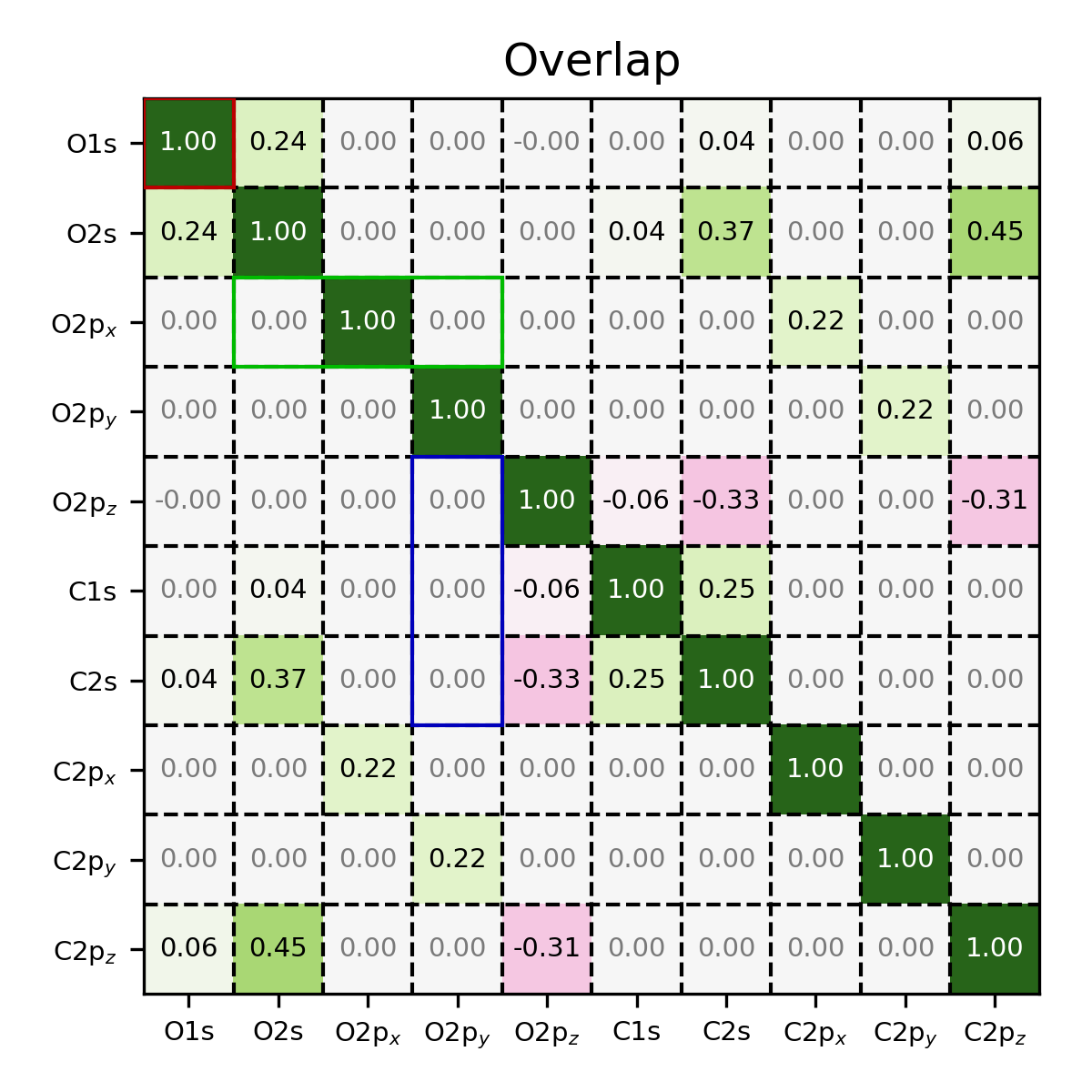
Coefficient matrix of CO, visualized using the MatrixPlotter class,
where a number of elements have been highlighted.
Note
The (x, y) coordinates use zero-based indexing. Consequently, the
top-left corner of the first box is specified as (0, 0).