Electronic structure calculations 

The PyQInt package provides two flavors of Hartree-Fock electronic structure calculations: restricted Hartree-Fock (RHF) and unrestricted Hartree-Fock (UHF). The restricted formulation is suitable for closed-shell systems, whereas the unrestricted formulation allows for the treatment of open-shell systems with unpaired electrons.

Both approaches expose detailed intermediate results, allowing the user to inspect orbital coefficients, density matrices, Fock matrices, and energy contributions throughout the self-consistent field (SCF) procedure.

Restricted Hartree-Fock 

Below, an example of an restricted Hartree-Fock calculation is given.

from pyqint import PyQInt, MoleculeBuilder, HF
import numpy as np
import matplotlib.pyplot as plt
from mpl_toolkits.axes_grid1 import make_axes_locatable

def main():
    # calculate sto3g coefficients for h2o
    cgfs, coeff = calculate_co()

    # visualize orbitals
    fig, ax = plt.subplots(2,5, figsize=(12, 5), dpi=144)
    sz = 3
    for i in range(0,2):
        for j in range(0,5):
            dens = plot_wavefunction(cgfs, coeff[:,i*5+j], sz=sz)
            limit = max(abs(np.min(dens)), abs(np.max(dens)) )
            im = ax[i,j].contourf(dens, origin='lower',
              extent=[-sz, sz, -sz, sz], cmap='PiYG', vmin=-limit, vmax=limit,
              levels=11)
            im = ax[i,j].contour(dens, origin='lower', colors='black',
              extent=[-sz, sz, -sz, sz], vmin=-limit, vmax=limit,
              levels=11)
            ax[i,j].set_xlabel('x [Bohr]')
            ax[i,j].set_ylabel('z [Bohr]')
            ax[i,j].set_aspect('equal', adjustable='box')
            ax[i,j].set_xticks(np.linspace(-3,3, 7))
            ax[i,j].set_yticks(np.linspace(-3,3, 7))
            ax[i,j].grid(linestyle='--', alpha=0.5)
    plt.tight_layout()
    plt.show()

def calculate_co():
    mol = MoleculeBuilder.from_name('CO')

    result = HF(mol, 'sto3g').rhf()

    return result['cgfs'], result['orbc']

def plot_wavefunction(cgfs, coeff, sz=3.5):
    # build integrator
    integrator = PyQInt()

    # build grid
    x = np.linspace(-sz, sz, 150)
    z = np.linspace(-sz, sz, 150)
    xx, zz = np.meshgrid(x,z)
    yy = np.zeros(len(x) * len(z))
    grid = np.vstack([xx.flatten(), yy, zz.flatten()]).reshape(3,-1).T
    res = integrator.plot_wavefunction(grid, coeff, cgfs).reshape((len(z), len(x)))

    return res

if __name__ == '__main__':
    main()

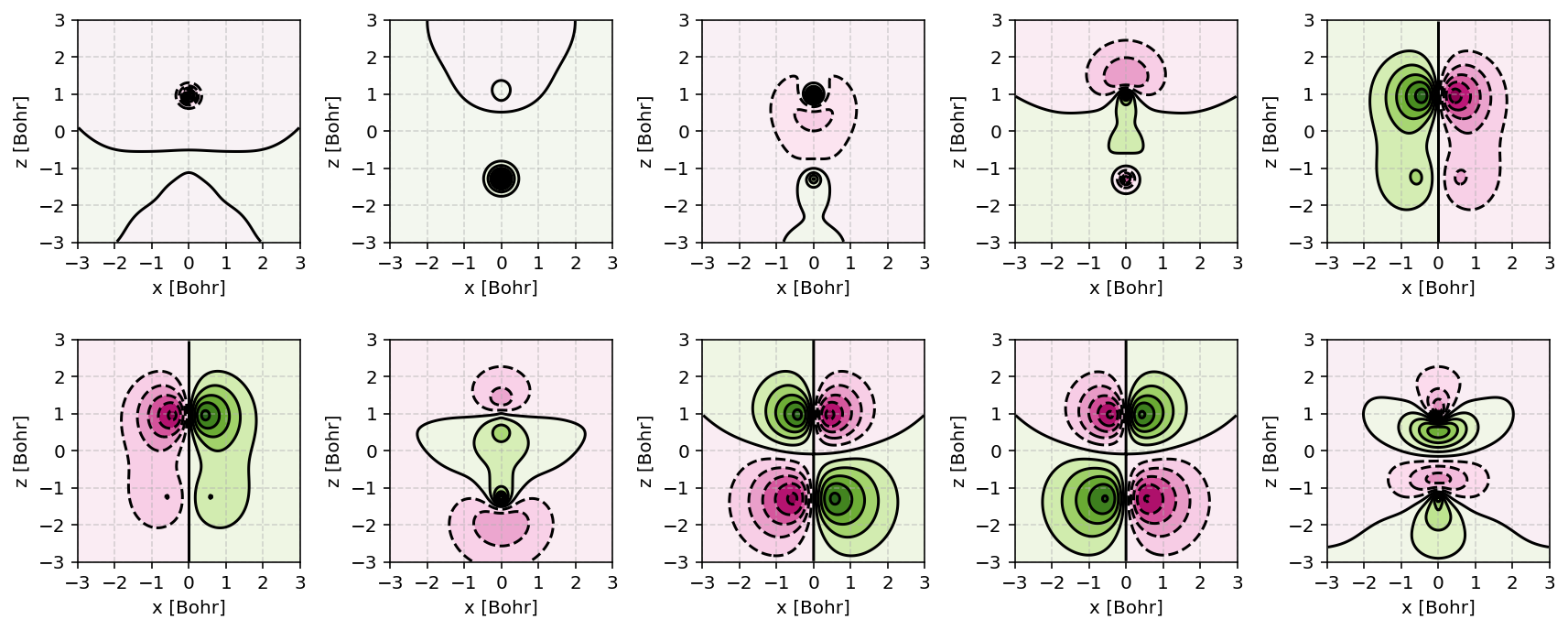
_images/co_orbs_contour.png — Canonical molecular orbitals of CO visualized using contour plots.

Hint

The manual construction of contour plots shown above provides full control over grid generation and visualization. For convenience, PyQInt also provides the ContourPlotter helper class (see ContourPlotter helper class) which encapsulates this workflow and allows rapid generation of grids of molecular orbital contour plots with minimal boilerplate code.

Result dictionary (RHF)

The result of a Hartree-Fock calculation is captured inside a dictionary object. This dictionary objects contains the following keys

Description of the data contained in the result library
Key	Description
`energy`	Final energy of the electronic structure calculation
`nuclei`	List of elements and their position in Bohr units
`cgfs`	List of contracted Gaussian functional objects
`energies`	List of energies during the self-convergence procedure
`orbe`	Orbital energies (converged) (array of N element)
`orbc`	Orbital coefficients (converted) (matrix of N x N elements)
`density`	Density matrix \(\mathbf{P}\)
`fock`	Fock matrix \(\mathbf{F}\)
`transform`	Unitary transformation matrix \(\mathbf{X}\)
`overlap`	Overlap matrix \(\mathbf{S}\)
`kinetic`	Kinetic energy matrix \(\mathbf{T}\)
`nuclear`	Nuclear attraction matrix \(\mathbf{V}\)
`hcore`	Core Hamiltonian matrix \(\mathbf{H_\textrm{core}}\)
`tetensor`	Two-electron tensor object \((i,j,k,l)\)
`time_stats`	Time statistics object
`ecore`	Sum of kinetic and nuclear attraction energy
`ekin`	Total kinetic energy
`enuc`	Total nuclear attraction energy
`erep`	Total electron-electron repulsion energy
`ex`	Total exchange energy
`enucrep`	Electrostatic repulsion energy of the nuclei
`nelec`	Total number of electrons
`mol`	Molecule class
`forces`	Forces on the atoms (if calculated, else `None`)

To provide an example how one can use the above data, let us consider the situation wherein the user wants to decompose the individual components of the total energy as given by

\[E_{\textrm{total}} = E_{\textrm{kin}} + E_{\textrm{nuc}} + E_{\textrm{e-e}} + E_{\textrm{ex}} + E_{\textrm{nuc,rep}}\]

Via the script below, one can easily verify that the above equation holds and that the total energy is indeed the sum of the kinetic, nuclear attraction, electron-electron repulsion, exchange and nuclear repulsion energies within a Hartree-Fock calculation.

from pyqint import MoleculeBuilder,HF

mol = MoleculeBuilder.from_name('ch4')
mol.name = 'CH4'

res = HF(mol, 'sto3g').rhf()
print()
print('Kinetic energy: ', res['ekin'])
print('Nuclear attraction energy: ', res['enuc'])
print('Electron-electron repulsion: ', res['erep'])
print('Exchange energy: ', res['ex'])
print('Repulsion between nuclei: ', res['enucrep'])
print()
print('Total energy: ', res['energy'])
print('Sum of the individual terms: ',
      res['ekin'] + res['enuc'] + res['erep'] + res['ex'] + res['enucrep'])

The output of the above script yields:

Kinetic energy:  39.42613774982387
Nuclear attraction energy:  -118.63789179775034
Electron-electron repulsion:  32.7324270326041
Exchange energy:  -6.609004673631048
Repulsion between nuclei:  13.362026647057352

Total energy:  -39.72630504189621
Sum of the individual terms:  -39.726305041896055

Unrestricted Hartree-Fock (UHF)

For systems containing unpaired electrons, such as radicals or atoms with open shells, the restricted Hartree-Fock approximation is no longer appropriate. In such cases, PyQInt provides an unrestricted Hartree-Fock (UHF) implementation via the uhf() method.

In UHF, separate spatial orbitals are used for spin-up (\(\alpha\)) and spin-down (\(\beta\)) electrons. This leads to distinct α and β density matrices and Fock matrices, allowing the electronic structure to exhibit spin polarization.

As a representative example, consider the methyl radical (CH₃), which has one unpaired electron and therefore requires an unrestricted treatment. The geometry used below places the carbon atom at the origin, with three hydrogen atoms arranged in a planar configuration with H-C-H angles of 120 degrees and a C-H bond length of 2.039 Bohr.

from pyqint import Molecule, HF
import numpy as np

R = 2.039
sqrt3 = np.sqrt(3.0)

mol = Molecule()
mol.add_atom('C', 0.0, 0.0, 0.0)
mol.add_atom('H',  R, 0.0, 0.0)
mol.add_atom('H', -0.5 * R,  0.5 * sqrt3 * R, 0.0)
mol.add_atom('H', -0.5 * R, -0.5 * sqrt3 * R, 0.0)

# CH3 is a doublet (multiplicity = 2)
res = HF(mol, 'sto3g').uhf(multiplicity=2)

print('Total energy:', res['energy'])

Result dictionary (UHF)

The result of an unrestricted Hartree-Fock (UHF) calculation is likewise captured inside a dictionary object. Compared to restricted Hartree-Fock, the UHF result dictionary contains spin-resolved quantities, reflecting the fact that different spatial orbitals are used for spin-up (\(\alpha\)) and spin-down (\(\beta\)) electrons.

Below, the most important entries of the UHF result dictionary are listed.

Description of the data contained in the UHF result dictionary
Key	Description
`energy`	Final total electronic energy
`nuclei`	List of elements and their position in Bohr units
`cgfs`	List of contracted Gaussian functional objects
`energies`	List of total energies during the SCF convergence procedure
`orbe_alpha`	Converged orbital energies for spin-up (\(\alpha\)) electrons
`orbe_beta`	Converged orbital energies for spin-down (\(\beta\)) electrons
`orbc_alpha`	Orbital coefficient matrix for \(\alpha\) electrons
`orbc_beta`	Orbital coefficient matrix for \(\beta\) electrons
`density_alpha`	Density matrix \(\mathbf{P}^{\alpha}\) for spin-up electrons
`density_beta`	Density matrix \(\mathbf{P}^{\beta}\) for spin-down electrons
`density`	Total density matrix \(\mathbf{P} = \mathbf{P}^{\alpha} + \mathbf{P}^{\beta}\)
`fock_alpha`	Fock matrix for \(\alpha\) electrons
`fock_beta`	Fock matrix for \(\beta\) electrons
`transform`	Unitary transformation matrix \(\mathbf{X}\)
`overlap`	Overlap matrix \(\mathbf{S}\)
`kinetic`	Kinetic energy matrix \(\mathbf{T}\)
`nuclear`	Nuclear attraction matrix \(\mathbf{V}\)
`hcore`	Core Hamiltonian matrix \(\mathbf{H_{\textrm{core}}}\)
`tetensor`	Two-electron integral tensor \((i,j,k,l)\)
`time_stats`	Time statistics object

In unrestricted Hartree-Fock, the exchange contribution is spin-dependent. Accordingly, the exchange energy is split into separate \(\alpha\) and \(\beta\) components.

UHF energy contributions
Key	Description
`ecore`	Sum of kinetic and nuclear attraction energy
`ej`	Coulomb (Hartree) energy
`ex_alpha`	Exchange energy contribution from \(\alpha\) electrons
`ex_beta`	Exchange energy contribution from \(\beta\) electrons
`enucrep`	Electrostatic repulsion energy of the nuclei

In addition to the electronic structure data, the UHF result dictionary contains explicit information about the spin state of the system.

Spin-related quantities
Key	Description
`nelec`	Total number of electrons
`nalpha`	Number of spin-up (\(\alpha\)) electrons
`nbeta`	Number of spin-down (\(\beta\)) electrons
`multiplicity`	Spin multiplicity \((2S + 1)\)

Note

Unlike restricted Hartree-Fock, unrestricted Hartree-Fock allows for spin polarization. As a consequence, the resulting wavefunction is generally not an exact eigenfunction of the total spin operator, which may lead to spin contamination.

Custom basis sets 

Besides the basis sets offered by PyQInt, one can also use a custom basis set defined by the user. The rhf routine accepts either a basis set for its basis argument, or alternatively a list of cgf objects. In the example code shown below, the latter is done.

from pyqint import Molecule, HF, cgf
mol = Molecule()
mol.add_atom('H', 0.0000, 0.0000, 0.3561150187, unit='angstrom')
mol.add_atom('H', 0.0000, 0.0000, -0.3561150187, unit='angstrom')
nuclei = mol.get_nuclei()

cgfs = []
for n in nuclei:
    cgf = CGF(n[0])

    cgf.add_gto(0.154329, 3.425251, 0, 0, 0)
    cgf.add_gto(0.535328, 0.623914, 0, 0, 0)
    cgf.add_gto(0.444635, 0.168855, 0, 0, 0)

    cgfs.append(cgf)

res = HF(mol, basis=cgfs).rhf(verbose=True)

Hint

A nice website to find a large collection of Gaussian Type basis set coefficients is https://www.basissetexchange.org/.

Electronic structure calculations

Restricted Hartree-Fock