Scalar field analysis

Once the electronic structure has been determined, a variety of scalar fields derived from the electron density can be analyzed and visualized. These fields provide insight into the spatial distribution of electronic properties and form the basis for interpreting exchange, correlation, and density-related quantities.

Electron density and its gradient

The pydft.DFT class exposes its internal matrices and a number of useful functions which we can readily use to interpret its operation. Let us start by generating a plot of the electron density using the method pydft.DFT.get_density_at_points().

import numpy as np
from pydft import MoleculeBuilder, DFT
import matplotlib.pyplot as plt
from mpl_toolkits.axes_grid1 import make_axes_locatable

# perform DFT calculation on the CO molecule
co = MoleculeBuilder().from_name("CO")
dft = DFT(co, basis='sto3g')
res = dft.scf(1e-6, verbose=False)

# generate grid of points and calculate the electron density for these points
sz = 4      # size of the domain
npts = 100  # number of sampling points per cartesian direction

# produce meshgrid for the xz-plane
x = np.linspace(-sz/2,sz/2,npts)
zz, xx = np.meshgrid(x, x, indexing='ij')
gridpoints = np.zeros((zz.shape[0], xx.shape[1], 3))
gridpoints[:,:,0] = xx
gridpoints[:,:,2] = zz
gridpoints[:,:,1] = np.zeros_like(xx) # set y-values to 0
gridpoints = gridpoints.reshape((-1,3))

# calculate (logarithmic) scalar field and convert if back to an 2D array
density = dft.get_density_at_points(gridpoints)
density = np.log10(density.reshape((npts, npts)))

# build contour plot
fig, ax = plt.subplots(1,1, dpi=144, figsize=(4,4))
im = ax.contourf(x, x, density, levels=np.linspace(-3,3,13, endpoint=True))
ax.contour(x, x, density, colors='black', levels=np.linspace(-3,3,13, endpoint=True))
ax.set_aspect('equal', 'box')
ax.set_xlabel('x-coordinate [a.u.]')
ax.set_ylabel('z-coordinate [a.u.]')
divider = make_axes_locatable(ax)
cax = divider.append_axes('right', size='5%', pad=0.05)
fig.colorbar(im, cax=cax, orientation='vertical')
ax.set_title('Electron density')
plt.show()

Running the above script yields the electron density.

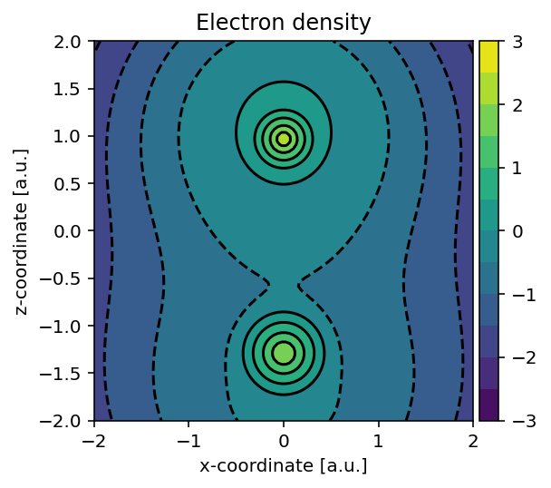
Logarithmic electron density of CO sampled in the molecular plane.

Using largely the same code, we can also readily build the electron density gradient magnitude using pydft.DFT.get_gradient_at_points().

import numpy as np
from pydft import MoleculeBuilder, DFT
import matplotlib.pyplot as plt
from mpl_toolkits.axes_grid1 import make_axes_locatable

# perform DFT calculation on the CO molecule
co = MoleculeBuilder().from_name("CO")
dft = DFT(co, basis='sto3g')
res = dft.scf(1e-6, verbose=False)

# generate grid of points and calculate the electron density for these points
sz = 4      # size of the domain
npts = 100  # number of sampling points per cartesian direction

# produce meshgrid for the xz-plane
x = np.linspace(-sz/2,sz/2,npts)
zz, xx = np.meshgrid(x, x, indexing='ij')
gridpoints = np.zeros((zz.shape[0], xx.shape[1], 3))
gridpoints[:,:,0] = xx
gridpoints[:,:,2] = zz
gridpoints[:,:,1] = np.zeros_like(xx) # set y-values to 0
gridpoints = gridpoints.reshape((-1,3))

# calculate (logarithmic) scalar field and convert if back to an 2D array
gradient = np.linalg.norm(dft.get_gradient_at_points(gridpoints), axis=1)
gradient = np.log10(gradient.reshape((npts, npts)))

# build contour plot
fig, ax = plt.subplots(1,1, dpi=144, figsize=(4,4))
im = ax.contourf(x, x, gradient, levels=np.linspace(-2,4,7, endpoint=True))
ax.contour(x, x, gradient, colors='black', levels=np.linspace(-2,4,7, endpoint=True))
ax.set_aspect('equal', 'box')
ax.set_xlabel('x-coordinate [a.u.]')
ax.set_ylabel('z-coordinate [a.u.]')
divider = make_axes_locatable(ax)
cax = divider.append_axes('right', size='5%', pad=0.05)
fig.colorbar(im, cax=cax, orientation='vertical')
ax.set_title('Electron density gradient magnitude')

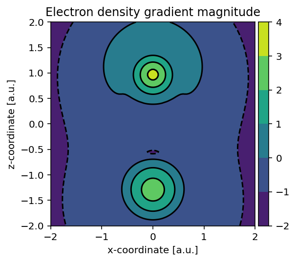
Magnitude of the electron-density gradient in the same plane.

Exchange potential

To construct the exchange potential at arbitrary grid points, we can use the script as shown below which uses the pydft.MolecularGrid.get_exchange_potential_at_points() method.

from pydft import DFT
from pyqint import MoleculeBuilder
import numpy as np
import matplotlib.pyplot as plt
from mpl_toolkits.axes_grid1 import make_axes_locatable

# perform DFT calculation on the CO molecule
co = MoleculeBuilder().from_name("CO")
dft = DFT(co, basis='sto3g')
res = dft.scf(1e-6, verbose=False)

# grab molecular orbital energies and coefficients
orbc = res['orbc']
orbe = res['orbe']

# generate grid of points and calculate the electron density for these points
sz = 4      # size of the domain
npts = 100  # number of sampling points per cartesian direction

# produce meshgrid for the xz-plane
x = np.linspace(-sz/2,sz/2,npts)
zz, xx = np.meshgrid(x, x, indexing='ij')
gridpoints = np.zeros((zz.shape[0], xx.shape[1], 3))
gridpoints[:,:,0] = xx
gridpoints[:,:,2] = zz
gridpoints[:,:,1] = np.zeros_like(xx) # set y-values to 0
gridpoints = gridpoints.reshape((-1,3))

# grab a copy of the MolecularGrid object
molgrid = dft.get_molgrid_copy()

# construct exchange potential
field = molgrid.get_exchange_potential_at_points(gridpoints, res['density'])
field = field.reshape((npts, npts))

# plot field
fig, ax = plt.subplots(1, 1, dpi=144, figsize=(4,4))
levels = np.linspace(-6,6,25, endpoint=True)
im = ax.contourf(x, x, field, levels=levels, cmap='PiYG')
ax.contour(x, x, field, levels=levels, colors='black', linewidths=0.5)
ax.set_aspect('equal', 'box')
ax.set_xlabel('x-coordinate [a.u.]')
ax.set_ylabel('z-coordinate [a.u.]')
divider = make_axes_locatable(ax)
cax = divider.append_axes('right', size='5%', pad=0.05)
fig.colorbar(im, cax=cax, orientation='vertical')
ax.set_title('Exchange potential')

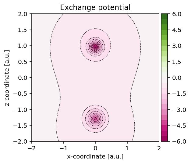
Exchange potential evaluated on an arbitrary two-dimensional grid.

Correlation potential

In a similar fashion as for the exchange potential, we can use the method pydft.MolecularGrid.get_correlation_potential_at_points() to obtain the correlation potential field.

from pydft import DFT
from pyqint import MoleculeBuilder
import numpy as np
import matplotlib.pyplot as plt
from mpl_toolkits.axes_grid1 import make_axes_locatable

# perform DFT calculation on the CO molecule
co = MoleculeBuilder().from_name("CO")
dft = DFT(co, basis='sto3g')
res = dft.scf(1e-6, verbose=False)

# grab molecular orbital energies and coefficients
orbc = res['orbc']
orbe = res['orbe']

# generate grid of points and calculate the electron density for these points
sz = 4      # size of the domain
npts = 100  # number of sampling points per cartesian direction

# produce meshgrid for the xz-plane
x = np.linspace(-sz/2,sz/2,npts)
zz, xx = np.meshgrid(x, x, indexing='ij')
gridpoints = np.zeros((zz.shape[0], xx.shape[1], 3))
gridpoints[:,:,0] = xx
gridpoints[:,:,2] = zz
gridpoints[:,:,1] = np.zeros_like(xx) # set y-values to 0
gridpoints = gridpoints.reshape((-1,3))

# grab a copy of the MolecularGrid object
molgrid = dft.get_molgrid_copy()

# construct correlation potential
field = molgrid.get_correlation_potential_at_points(gridpoints, res['density'])
field = field.reshape((npts, npts))

# plot field
fig, ax = plt.subplots(1, 1, dpi=144, figsize=(4,4))
levels = np.linspace(-0.2,0.2,101, endpoint=True)
im = ax.contourf(x, x, field, levels=levels, cmap='PiYG')
ax.contour(x, x, field, levels=levels, colors='black', linewidths=0.5)
ax.set_aspect('equal', 'box')
ax.set_xlabel('x-coordinate [a.u.]')
ax.set_ylabel('z-coordinate [a.u.]')
divider = make_axes_locatable(ax)
cax = divider.append_axes('right', size='5%', pad=0.05)
fig.colorbar(im, cax=cax, orientation='vertical')
ax.set_title('Correlation potential')

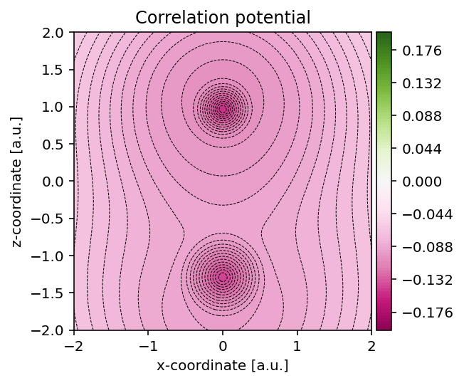
Correlation potential evaluated on the same grid.