Hartree potential analysis
The Hartree potential is calculated from the electron density distribution using the Poisson equation [Becke and Dickson, 1988].
PyDFT solves this problem in an atom-centered representation. The molecular density is first split into Becke fuzzy cells. Within each cell, the angular dependence is expanded in real spherical harmonics, leaving a set of radial equations that can be solved numerically. The resulting coefficients are later interpolated back to the full molecular grid to assemble the Coulomb matrix.
Projection onto spherical harmonics
The Poisson equation is solved on the atomic grid by first projecting the electron density onto the spherical harmonics such that the following equation holds.
where \(\rho(r_{k}, \Omega)\) is the electron density at radius \(r_{k}\), \(\rho_{klm}\) the linear expansion coefficient at position \(r_{k}\) for the spherical harmonic \(lm\) and \(Y_{lm}\) a spherical harmonic with quantum numbers \(l\) and \(m\).
We can readily visualize and interpret this projection using the
pydft.MolecularGrid.get_rho_lm_atoms() as shown by the script below.
 1import numpy as np
 2from pydft import MoleculeBuilder, DFT
 3import matplotlib.pyplot as plt
 4from mpl_toolkits.axes_grid1 import make_axes_locatable
 5
 6def main():
 7    # perform DFT calculation on the CO molecule
 8    co = MoleculeBuilder().from_name("CO")
 9    dft = DFT(co, basis='sto3g')
10    res = dft.scf(1e-6, verbose=False)
11
12    # get the projection onto the spherical harmonics
13    lmprojection = dft.get_molgrid_copy().get_rho_lm_atoms()
14
15    fig, ax = plt.subplots(1, 2, dpi=144, figsize=(6,4))
16    plot_spherical_harmonic_projection(ax[1], fig, lmprojection[0], title='O')
17    plot_spherical_harmonic_projection(ax[0], fig, lmprojection[1], title='C')
18    plt.tight_layout()
19
20def plot_spherical_harmonic_projection(ax, fig, mat, minval=5e-2, title=None):
21    im = ax.imshow(np.flip(mat, axis=0), origin='lower', cmap='PiYG', vmin=-minval,vmax=minval)
22    ax.grid(linestyle='--', color='black', alpha=0.8)
23    ax.set_xticks([-0.5,0.5,3.5,8.5,15.5], labels=['s','p','d','f','g'])
24    ax.set_yticks(np.arange(0, mat.shape[0], 5)-0.5,
25                  labels=np.arange(0, mat.shape[0], 5))
26    ax.set_ylabel('Radial points $r_{i}$')
27    ax.set_xlim(-.5,15)
28    ax.set_xlabel('Spherical harmonics (lm)')
29    divider = make_axes_locatable(ax)
30    cax = divider.append_axes('right', size='5%', pad=0.05)
31    fig.colorbar(im, cax=cax, orientation='vertical')
32
33    if title is not None:
34        ax.set_title(title)
35
36if __name__ == '__main__':
37    main()
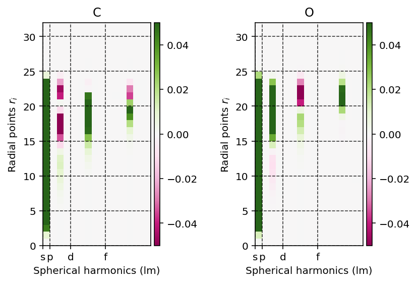
Spherical-harmonic expansion coefficients of the atom-centered density.
Radial Poisson solve
After the density coefficients \(\rho_{klm}\) have been constructed, PyDFT solves a finite-difference form of the radial Poisson equation for each \((l,m)\) channel. The solution is stored as Hartree-potential expansion coefficients \(U_{klm}\) on the radial grid of each atom.
During an SCF calculation the density changes at every iteration, so these coefficients also change. The geometry of the interpolation problem, however, does not change: the molecular grid points remain at the same distances from each atomic center. PyDFT therefore precomputes cubic interpolation stencils once and reuses them when the updated \(U_{klm}\) values are needed on the molecular grid.
Coulomb matrix assembly
Once the Hartree potential is known on the molecular grid, the Coulomb matrix is obtained by numerical quadrature over products of basis functions:
In the code, this final step is performed by
pydft.MolecularGrid.calculate_coulombic_matrix().