Electronic Structure Calculations

To start, we perform a high-level calculation of the electronic structure of the carbon-monoxide molecule using the default SVWN5 exchange-correlation functional [Slater, 1951, Vosko et al., 1980]. To perform this calculation, we first have to construct a pydft.DFT object which requires a molecule as its input. Next, we use the pydft.DFT.scf() routine to start the self-consistent field calculation.

from pydft import MoleculeBuilder, DFT

# perform DFT calculation on the CO molecule
co = MoleculeBuilder().from_name("CO")
dft = DFT(co, basis='sto3g')
res = dft.scf(1e-6, verbose=False)

# print total energy
print("Total electronic energy:     %12.6f Ht" % res['energy'])

Performing this calculation shows that the total electronic energy for this system corresponds to:

Total electronic energy:      -111.130470 Ht

Result dictionary

The result of an SCF calculation is captured in a Python dictionary object. This dictionary contains all quantities required to analyze, post-process, and validate the electronic structure calculation. The data layout is shared between PyDFT and PyQInt to ensure a consistent interface across methods.

The most commonly used key is energy, which stores the final converged total energy. Other entries expose the objects that appear in the SCF equations: the density matrix \(\mathbf{P}\), the one-electron matrices \(\mathbf{S}\), \(\mathbf{T}\), and \(\mathbf{V}\), the Hartree matrix \(\mathbf{J}\), and the exchange-correlation matrix. This is why examples usually store the SCF result as res and then access quantities such as res['energy'] or res['density'].

Description of the data contained in the result dictionary

Key	Description
energy	Final converged total electronic energy (Hartree).
energies	Total electronic energy at each SCF iteration.
ekin	Electronic kinetic energy, \(\mathrm{Tr}(\mathbf{T}\mathbf{P})\).
enuc	Electron-nuclear attraction energy, \(\mathrm{Tr}(\mathbf{V}\mathbf{P})\).
erepe	Electron-electron Coulomb (Hartree) energy, \(\mathrm{Tr}(\mathbf{J}\mathbf{P})\).
enucrep	Nuclear-nuclear repulsion energy.
ex	Exchange energy (Hartree-Fock or DFT).
ec	Correlation energy (DFT only).
exc	Total exchange-correlation energy.
orbe	Molecular orbital eigenvalues (orbital energies).
orbc	Molecular orbital coefficient matrix (AO basis).
density	One-particle density matrix \(\mathbf{P}\).
fock	Fock matrix \(\mathbf{F}\).
hartree	Hartree (Coulomb) matrix \(\mathbf{J}\).
xc	Exchange-correlation matrix (DFT only, None for HF).
overlap	Overlap matrix \(\mathbf{S}\).
kinetic	Kinetic energy matrix \(\mathbf{T}\).
nuclear	Nuclear attraction matrix \(\mathbf{V}\).
hcore	Core Hamiltonian matrix \(\mathbf{H}_\mathrm{core} = \mathbf{T} + \mathbf{V}\).
mol	Molecular object defining atoms, geometry, and charge.
nuclei	Nuclear positions and charges.
cgfs	List of contracted Gaussian basis functions.
nelec	Total number of electrons.
time_stats	Dictionary containing timing information for construction and SCF iterations.

Energy decomposition

The molecular matrices can be used to perform a so-called energy decomposition, i.e., decompose the total electronic energy into the kinetic, nuclear attraction, electron-electron repulsion and exchange-correlation energy.

import numpy as np
from pydft import MoleculeBuilder, DFT

co = MoleculeBuilder().from_name("CO")
dft = DFT(co, basis='sto3g')
res = dft.scf(1e-4, verbose=False)
print("Total electronic energy:     %12.6f Ht" % res['energy'])
print()

# retrieve molecular matrices
P = res['density']
T = res['kinetic']
V = res['nuclear']
J = res['hartree']

# calculate energy terms
Et = np.einsum('ji,ij', P, T)
Ev = np.einsum('ji,ij', P, V)
Ej = 0.5 * np.einsum('ji,ij', P, J)
Ex = res['ex']
Ec = res['ec']
Exc = res['exc']
Enuc = res['enucrep']

print('Kinetic energy:              %12.6f Ht' % Et)
print('Nuclear attraction:          %12.6f Ht' % Ev)
print('Electron-electron repulsion: %12.6f Ht' % Ej)
print('Exchange energy:             %12.6f Ht' % (Ex))
print('Correlation energy:          %12.6f Ht' % (Ec))
print('Exchange-correlation energy: %12.6f Ht' % (Exc))
print('Nucleus-nucleus repulsion:   %12.6f Ht' % (Enuc))
print()
print('Sum: %12.6f Ht' % (Et + Ev + Ej + Exc + Enuc))

The above script yields the following output:

Total electronic energy:      -111.130470 Ht

Kinetic energy:                110.217226 Ht
Nuclear attraction:           -304.930911 Ht
Electron-electron repulsion:    75.612987 Ht
Exchange energy:               -12.055233 Ht
Correlation energy:             -1.232632 Ht
Exchange-correlation energy:   -13.287865 Ht
Nucleus-nucleus repulsion:      21.258092 Ht

Sum:  -111.130470 Ht

Self-consistent field matrices

To visualize the overlap matrix \(\mathbf{S}\) and the Fock matrix \(\mathbf{F}\), we can use the script as found below.

import numpy as np
from pydft import MoleculeBuilder, DFT
import matplotlib.pyplot as plt

def main():
    # perform DFT calculation on the CO molecule
    co = MoleculeBuilder().from_name("CO")
    dft = DFT(co, basis='sto3g')
    res = dft.scf(1e-6, verbose=False)
    
    # build list of basis functions
    labels = []
    for a in co.get_atoms():
        for o in ['1s', '2s', '2px', '2py', '2pz']:
            labels.append('%s - %s' % (a[0],o))
    
    fig, ax = plt.subplots(1, 2, dpi=144, figsize=(8,4))
    plot_matrix(ax[0], res['overlap'], xlabels=labels, ylabels=labels, title='Overlap matrix')
    plot_matrix(ax[1], res['fock'], xlabels=labels, ylabels=labels, title='Hamiltonian matrix')

def plot_matrix(ax, mat, xlabels=None, ylabels=None, title = None, xlabelrot=90):
    """
    Produce plot of matrix
    """
    ax.imshow(mat, vmin=-1, vmax=1, cmap='PiYG')
    for i in range(mat.shape[0]):
        for j in range(mat.shape[1]):
            ax.text(i, j, '%.2f' % mat[j,i], ha='center', va='center',
                    fontsize=7)
    ax.set_xticks([])
    ax.set_yticks([])
    ax.hlines(np.arange(1, mat.shape[0])-0.5, -0.5, mat.shape[0] - 0.5,
              color='black', linestyle='--', linewidth=1)
    ax.vlines(np.arange(1, mat.shape[0])-0.5, -0.5, mat.shape[0] - 0.5,
              color='black', linestyle='--', linewidth=1)
    
    ax.set_xticks(np.arange(0, mat.shape[0]))
    if xlabels is not None:
        ax.set_xticklabels(xlabels, rotation=xlabelrot)
    ax.set_yticks(np.arange(0, mat.shape[0]))
    
    if ylabels is not None:
        ax.set_yticklabels(ylabels, rotation=0)
    ax.tick_params(axis='both', which='major', labelsize=7)
    
    if title is not None:
        ax.set_title(title)

if __name__ == '__main__':
    main()

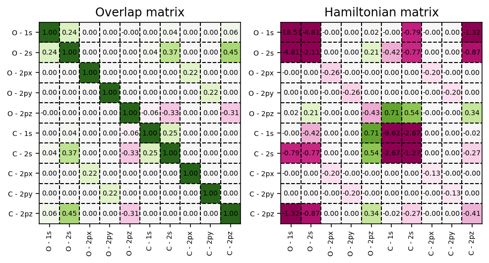
Overlap and Hamiltonian matrices exposed by the SCF result dictionary.

Showing the electronic steps

To get verbose output, i.e. information per electronic step, configure logging and specify verbose = True.

Note

PyDFT uses Python’s standard logging module for these progress messages instead of printing directly. This means that verbose = True tells PyDFT to create informational log messages, while logging.basicConfig(...) tells Python where and how to show them. Without the logging configuration, the calculation still runs normally, but the progress messages remain hidden. This makes it possible to use PyDFT quietly in scripts, tests, and notebooks, or to send messages to the terminal when interactive feedback is useful.

import logging

from pydft import MoleculeBuilder, DFT

logging.basicConfig(level=logging.INFO, format="%(message)s")

# perform DFT calculation on the CO molecule
co = MoleculeBuilder().from_name("CO")
dft = DFT(co, basis='sto3g')
res = dft.scf(1e-5, verbose=True)

Executing the script above yields output like the following. The timings depend on the machine and runtime environment:

001 | E =  -179.237419 | dE = 0.0000e+00 | 0.0010 s
002 | E =  -106.662588 | dE = 0.0000e+00 | 1.2765 s
003 | E =  -117.641796 | dE = 7.2575e+01 | 0.0172 s
004 | E =  -107.190988 | dE = 1.0979e+01 | 0.0201 s
005 | E =  -117.376118 | dE = 1.0451e+01 | 0.0203 s
006 | E =  -117.085797 | dE = 1.0185e+01 | 0.0160 s
007 | E =  -108.013652 | dE = 2.9032e-01 | 0.0149 s
008 | E =  -107.421366 | dE = 9.0721e+00 | 0.0143 s
009 | E =  -110.457951 | dE = 5.9229e-01 | 0.0151 s
010 | E =  -110.419024 | dE = 3.0366e+00 | 0.0176 s
011 | E =  -109.548780 | dE = 3.8927e-02 | 0.0159 s
012 | E =  -111.008079 | dE = 8.7024e-01 | 0.0159 s
013 | E =  -111.118875 | dE = 1.4593e+00 | 0.0163 s
014 | E =  -111.130700 | dE = 1.1080e-01 | 0.0162 s
015 | E =  -111.130454 | dE = 1.1825e-02 | 0.0210 s
016 | E =  -111.130470 | dE = 2.4610e-04 | 0.0258 s
017 | E =  -111.130470 | dE = 1.6288e-05 | 0.0188 s
018 | E =  -111.130470 | dE = 9.2335e-08 | 0.0158 s
Stopping SCF cycle, convergence reached.

Each line corresponds to one update of the density matrix. Internally, PyDFT uses the current density matrix to build the electron density on the molecular grid, constructs the Hartree and exchange-correlation matrices, forms the Kohn-Sham/Fock matrix, diagonalizes it, and then builds the next density matrix from the occupied orbitals. The energy difference dE is the convergence measure used by pydft.DFT.scf().

Different exchange-correlation functionals

To use a different exchange-correlation functional, pass the functional argument when constructing the pydft.DFT object:

from pydft import MoleculeBuilder, DFT

# perform DFT calculation on the CO molecule
co = MoleculeBuilder().from_name("CO")

# use SVWN XC functional
dft = DFT(co, basis='sto3g', functional='svwn5')
print('SVWN: ', dft.scf(1e-5)['energy'], 'Ht')

# use PBE XC functional
dft = DFT(co, basis='sto3g', functional='pbe')
print('PBE: ', dft.scf(1e-5)['energy'], 'Ht')

which yields the following total electronic energies for the SVWN5 and PBE [Perdew et al., 1996] exchange-correlation functions:

SVWN:  -111.13047044798054 Ht
PBE:  -111.64036457334683 Ht

Tuning the numerical accuracy

The numerical accuracy of an electronic structure calculation in PyDFT can be controlled through the specification of the radial and angular integration grids. These grids are defined per atomic species and can be adjusted by the user when constructing the pydft.DFT object.

The radial grid is controlled via the number of radial shells (nshells), while the angular resolution is controlled via the number of angular points (nangpts). Both parameters are provided as mappings from element symbols to integer values. Increasing either parameter generally improves the accuracy of the numerical integration at the cost of increased computational effort.

The angular grid in PyDFT is based on Lebedev quadrature. As a consequence, the number of angular points must correspond to one of the predefined Lebedev grid sizes [Lebedev, 1976]. Arbitrary values for nangpts are not permitted; only the fixed values listed below are valid.

The supported numbers of angular points are:

6, 14, 26, 38, 50, 74, 86, 110, 146, 170, 194, 230,
266, 302, 350, 434, 590, 770, 974, 1202, 1454, 1730,
2030, 2354, 2702, 3074, 3470, 3890, 4334, 4802,
5294, 5810

By default, PyDFT uses 20, 25, and 30 radial shells for first-, second-, and third-row atoms, respectively. For the angular grid, 110 angular points are used for all atoms, except for hydrogen, for which 50 angular points are used. The maximum angular momentum quantum number lmax is determined automatically from the chosen number of angular points; for the default values, this corresponds to lmax = 8 for 110 angular points and lmax = 5 for 50 angular points.

Users may override these defaults by explicitly specifying nshells and nangpts when constructing the pydft.DFT object. For example, a calculation with a moderately accurate grid can be set up as

from pydft import MoleculeBuilder, DFT

mol = MoleculeBuilder().from_name("CO")
dft = DFT(mol, basis='sto3g',
    nshells={'C': 32, 'O': 32},
    nangpts={'C': 230, 'O': 230}
)
res = dft.scf(1e-6, verbose=False)

print("Total electronic energy:     %12.6f Ht" % res['energy'])

which shows the following output:

Total electronic energy:      -111.142418 Ht

If higher accuracy is required, the number of radial shells can be increased, for example to 64, and the number of angular points can be increased by selecting a larger Lebedev grid from the list above. In practice, we observe that increasing the number of angular points beyond a certain threshold does not lead to significant further improvements in accuracy, whereas increasing the number of radial shells continues to systematically reduce the error.

By adjusting nshells and selecting an appropriate Lebedev grid via nangpts, users can balance computational cost and numerical accuracy according to the requirements of their specific application.