Background
PyDFT is a pure-Python package for performing Density Functional Theory (DFT) calculations. It builds on top of PyQInt, which handles the underlying quantum-chemical integrals, and draws on PyLebedev for numerical integration on the unit sphere and PyTessel for generating isosurfaces of molecular orbitals.
The goal of PyDFT is not to be the fastest DFT code, but to be the most transparent one. Every intermediate quantity, including the molecular grid, the electron density, the Hartree and exchange-correlation potentials, the matrix elements, and the orbital energies, is accessible and can be inspected, plotted, or modified. This makes it well suited for learning how a DFT calculation is actually assembled.
Tip
A detailed explanation of the theory behind PyDFT can be found in the textbook “Elements of Electronic Structure Theory” (chapter 4), which is freely available via this website.
Overview of the PyDFT workflow
The figure below gives a bird’s-eye view of a complete PyDFT calculation. It is divided into four stages that mirror the sections of this page.
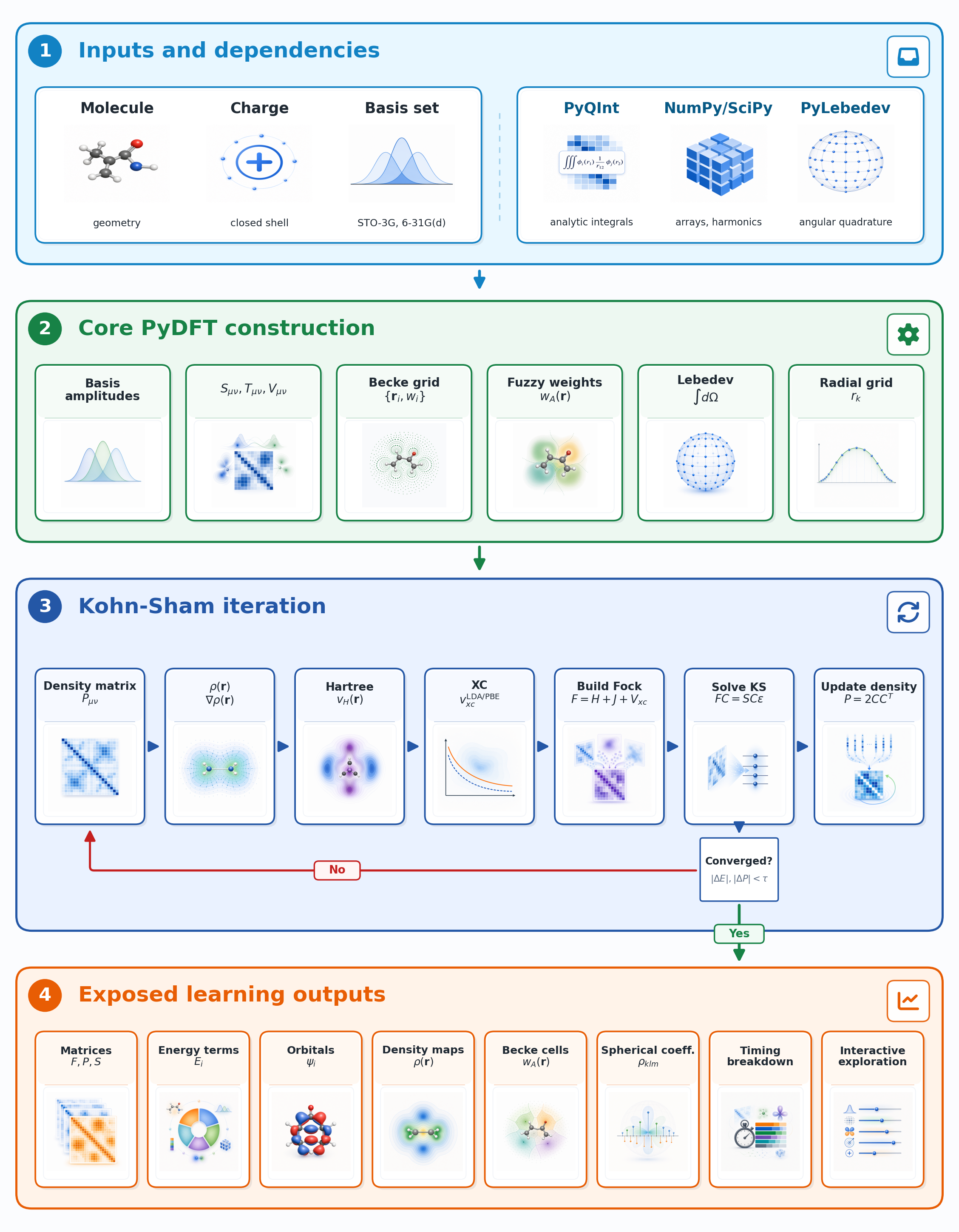
High-level overview of the PyDFT workflow. Molecular input, charge, and basis-set information are combined with PyQInt, NumPy, and PyLebedev to construct the numerical objects required by PyDFT. The package then builds atom-centered Becke grids, evaluates densities and potentials, iterates the restricted Kohn-Sham equations to self-consistency, and exposes intermediate matrices, fields, orbitals, energy components, and timing data for educational inspection.
Inputs and dependencies. The user provides a molecular geometry, a charge (which determines whether the system is neutral or ionic), and a choice of Gaussian basis set. PyQInt takes these and computes all the one-electron integrals needed to build the Hamiltonian. PyLebedev provides the angular quadrature points on the unit sphere that are used later to build the numerical grid.
Core PyDFT construction. PyDFT evaluates the basis-function amplitudes at every grid point, assembles the one-electron matrices (overlap \(\mathbf{S}\), kinetic energy \(\mathbf{T}\), nuclear attraction \(\mathbf{V}\)), and constructs the atom-centered Becke grid together with the fuzzy-cell weights.
Kohn-Sham iteration. The core of the calculation is a self-consistent field (SCF) loop: starting from an initial guess for the electron density, PyDFT builds the Fock matrix, solves the Kohn-Sham equations for new orbitals, and updates the density. This repeats until the density no longer changes appreciably between cycles.
Exposed learning outputs. Once converged, the full range of quantities is available for inspection: matrices, energy terms, orbitals, density maps, Becke cells, spherical-harmonic coefficients, timing data, and more.
From molecule to basis set
Every DFT calculation starts with a description of the molecule: the nuclear positions, the atomic numbers, and the total charge. From these, a basis set is chosen, that is, a collection of Gaussian-type functions (GTOs) centred on the atoms. These functions serve as the building blocks with which the electronic wave function will be approximated; a larger basis set gives a more flexible description of the electrons but also makes the calculation more expensive.
PyDFT delegates all basis-set and integral work to PyQInt. It computes the three one-electron matrices that appear in any quantum-chemical method:
the overlap matrix \(\mathbf{S}\), which measures how much each pair of basis functions overlaps in space;
the kinetic-energy matrix \(\mathbf{T}\), which encodes the kinetic energy of electrons moving through the basis;
the nuclear-attraction matrix \(\mathbf{V}\), which describes the attraction of the electrons to the nuclei.
Together these form the one-electron Hamiltonian \(\mathbf{H}^{\text{core}} = \mathbf{T} + \mathbf{V}\), which is the starting point for the Kohn-Sham procedure.
Molecular decomposition and numerical grid
A DFT calculation requires evaluating many integrals over three-dimensional space, for example to compute the electron density or the energy. These integrals are almost never solved analytically; instead, PyDFT uses numerical integration, also called quadrature.
The key idea is to break the molecule apart into a set of overlapping, atom-centered regions, often called fuzzy cells. Each atom gets its own region of space, and the boundaries between regions are kept deliberately smooth so that nothing is double-counted. This approach, introduced by Becke [Becke, 1988], turns one difficult molecular integral into a sum of simpler atom-by-atom integrals.
PyDFT builds a grid around each atom using two components: a
radial Gauss-Chebyshev grid that samples distances from the nucleus, and
an angular Lebedev grid [Lebedev, 1976] that samples directions on a
sphere. The Becke partitioning then assigns a smooth weight to each grid
point, indicating how much that point “belongs” to a given atom. Because the
weights sum to one everywhere, the full molecular integral is recovered
exactly as a weighted sum over all atomic grids. In the code, the
molecular-level grid is managed by pydft.MolecularGrid and the
per-atom grids by pydft.AtomicGrid.
The Kohn-Sham self-consistent field loop
The central idea of Kohn-Sham DFT [Kohn and Sham, 1965] is to replace the interacting many-electron problem with an equivalent system of non-interacting electrons that produce the same ground-state electron density. These fictitious non-interacting electrons move in an effective potential, the Kohn-Sham potential, which combines the external potential of the nuclei, the classical electron-electron repulsion (the Hartree term), and a correction for all quantum-mechanical many-body effects (the exchange-correlation term).
Because the Kohn-Sham potential itself depends on the electron density, and the density depends on the orbitals, and the orbitals depend on the potential, the problem must be solved self-consistently. In practice this means running an iterative loop:
Initialize. Start with an initial guess for the electron density \(\rho\), typically built from a superposition of atomic densities.
Build the Kohn-Sham (Fock) matrix \(\mathbf{F}\). This involves computing the Hartree potential \(V_H[\rho]\) and the exchange-correlation potential \(V_{xc}[\rho]\) on the numerical grid and integrating them with pairs of basis functions.
Solve the Kohn-Sham equations \(\mathbf{FC} = \mathbf{SC}\mathbf{\varepsilon}\). This is a generalized eigenvalue problem whose solutions are the orbital coefficient matrix \(\mathbf{C}\) and the orbital energies \(\varepsilon\).
Update the density matrix \(\mathbf{P} = 2\mathbf{C}_{\text{occ}}\mathbf{C}_{\text{occ}}^T\), where the factor of 2 accounts for spin in a closed-shell system.
Check convergence. If the density has changed by less than a threshold between cycles, the calculation is finished. Otherwise, return to step 2 with the new density (optionally mixed with the old density to help convergence).
PyDFT supports density mixing and DIIS (Direct Inversion of the Iterative Subspace) [Pulay, 1980] to accelerate and stabilize convergence. Once the loop has converged, the total electronic energy is assembled from kinetic, nuclear-attraction, Hartree, and exchange-correlation contributions.
Hartree potential
When electrons repel one another, each electron feels an electrostatic potential created by the charge distribution of all the other electrons. This is called the Hartree potential, and computing it accurately is one of the more challenging steps in a DFT calculation.
PyDFT obtains the Hartree potential by solving Poisson’s equation, the classical equation that relates a charge distribution to the electrostatic potential it produces. Following the method of Becke and Dickson [Becke and Dickson, 1988], this is done separately for each fuzzy cell, which keeps the problem tractable.
The procedure works in stages that are easy to follow: the electron density in each atomic cell is first expanded in terms of real spherical harmonics (think of these as angular “shape functions” on a sphere). Poisson’s equation is then solved independently for each angular channel, giving a set of radial Hartree-potential coefficients. These coefficients are interpolated back onto the full molecular grid, and the result is integrated with pairs of basis functions to assemble the Coulomb matrix \(\mathbf{J}\).
Exchange-correlation functions
In DFT, the exchange-correlation functional captures quantum-mechanical effects, most importantly the fact that electrons of the same spin avoid each other (exchange) and that electron motion is correlated. This part of the energy cannot be computed exactly and must be approximated.
PyDFT currently supports two widely-used approximations:
LDA (Local Density Approximation): combines Slater exchange [Slater, 1951] with the SVWN5 correlation functional [Vosko et al., 1980]. The energy density at each point depends only on the local electron density \(\rho\) at that point. This is the simplest meaningful approximation and a good starting point for learning DFT.
PBE (Perdew-Burke-Ernzerhof): a Generalised Gradient Approximation (GGA) functional [Perdew et al., 1996]. It improves on LDA by also taking into account how the density varies spatially through the gradient invariant \(\sigma = |\nabla\rho|^2\). This extra information makes PBE more accurate for most molecules, at a modest additional cost.
Both functionals are evaluated on the numerical molecular grid. For PBE, PyDFT also caches the basis-function gradients needed to evaluate \(\sigma\) and adds the corresponding GGA contribution to the exchange-correlation matrix.
What you can inspect
A key design goal of PyDFT is that intermediate quantities are not hidden. After a converged calculation, the following objects are directly accessible through the Python interface:
Matrices: the overlap, kinetic-energy, nuclear-attraction, Hartree, exchange-correlation, and full Kohn-Sham (Fock) matrices.
Energy decomposition: the total energy broken into its kinetic, nuclear-attraction, Hartree, and exchange-correlation components.
Orbitals and orbital energies: the coefficient matrix \(\mathbf{C}\) and the Kohn-Sham eigenvalues \(\varepsilon_i\).
Density fields: the electron density \(\rho(\mathbf{r})\) and, for GGA calculations, its gradient \(|\nabla\rho|\) on the molecular grid.
Becke cells and weights: the fuzzy-cell decomposition of the molecule, useful for visualizing the grid and understanding numerical integration.
Hartree and XC potentials: the potentials as scalar fields on the grid.
Spherical-harmonic coefficients: the expansion of the density used inside the Hartree solver.
Timing data: per-step wall times, useful for understanding where computation time is spent as grid resolution is varied.
The tutorials in this documentation walk through each of these in detail, with code examples and visualizations.