Orbital Visualization

Within the Kohn-Sham approximation, the set of molecular orbitals that minimizes the total electronic energy are found via the diagonalization of the Fock matrix.

Coefficient matrix

These Kohn-Sham orbitals are encoded in the coefficient matrix which is extracted via the script below.

import numpy as np
from pydft import MoleculeBuilder, DFT
import matplotlib.pyplot as plt

def main():
    # perform DFT calculation on the CO molecule
    co = MoleculeBuilder().from_name("CO")
    dft = DFT(co, basis='sto3g')
    res = dft.scf(1e-6, verbose=False)
    
    # build list of basis functions
    labels = []
    for a in co.get_atoms():
        for o in ['1s', '2s', '2px', '2py', '2pz']:
            labels.append('%s - %s' % (a[0],o))
    
    fig, ax = plt.subplots(1, 1, dpi=144, figsize=(4,4))
    plot_matrix(ax, res['orbc'], xlabels=[str(i) for i in np.arange(1,11)],
                ylabels=labels, title='Coefficient matrix')

def plot_matrix(ax, mat, xlabels=None, ylabels=None, title = None, xlabelrot=90):
    """
    Produce plot of matrix
    """
    ax.imshow(mat, vmin=-1, vmax=1, cmap='PiYG')
    for i in range(mat.shape[0]):
        for j in range(mat.shape[1]):
            ax.text(i, j, '%.2f' % mat[j,i], ha='center', va='center',
                    fontsize=7)
    ax.set_xticks([])
    ax.set_yticks([])
    ax.hlines(np.arange(1, mat.shape[0])-0.5, -0.5, mat.shape[0] - 0.5,
              color='black', linestyle='--', linewidth=1)
    ax.vlines(np.arange(1, mat.shape[0])-0.5, -0.5, mat.shape[0] - 0.5,
              color='black', linestyle='--', linewidth=1)
    
    ax.set_xticks(np.arange(0, mat.shape[0]))
    if xlabels is not None:
        ax.set_xticklabels(xlabels, rotation=xlabelrot)
    ax.set_yticks(np.arange(0, mat.shape[0]))
    
    if ylabels is not None:
        ax.set_yticklabels(ylabels, rotation=0)
    ax.tick_params(axis='both', which='major', labelsize=7)
    
    if title is not None:
        ax.set_title(title)

if __name__ == '__main__':
    main()

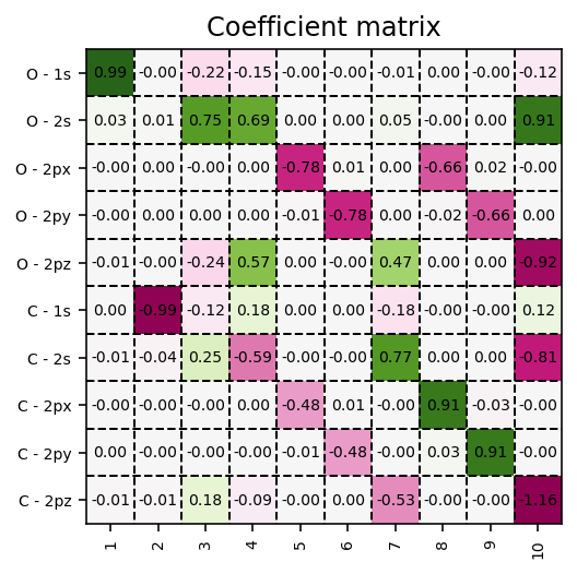
Molecular-orbital coefficient matrix in the atomic-orbital basis.

Contour plots

These orbitals can be readily visualized, as exemplified in the code below. Here, we make use of the pydft.MolecularGrid.get_amplitude_at_points() method. To use this method, we first have to retrieve the pydft.MolecularGrid object from the pydft.DFT class via its pydft.DFT.get_molgrid_copy() method.

import numpy as np
from pydft import MoleculeBuilder, DFT
import matplotlib.pyplot as plt
from mpl_toolkits.axes_grid1 import make_axes_locatable

def main():
    # perform DFT calculation on the CO molecule
    co = MoleculeBuilder().from_name("CO")
    dft = DFT(co, basis='sto3g')
    res = dft.scf(1e-6, verbose=False)
    
    # grab molecular orbital energies and coefficients
    orbc = res['orbc']
    orbe = res['orbe']
    
    # generate grid of points and calculate the electron density for these points
    sz = 4      # size of the domain
    npts = 100  # number of sampling points per cartesian direction
    
    # produce meshgrid for the xz-plane
    x = np.linspace(-sz/2,sz/2,npts)
    zz, xx = np.meshgrid(x, x, indexing='ij')
    gridpoints = np.zeros((zz.shape[0], xx.shape[1], 3))
    gridpoints[:,:,0] = xx
    gridpoints[:,:,2] = zz
    gridpoints[:,:,1] = np.zeros_like(xx) # set y-values to 0
    gridpoints = gridpoints.reshape((-1,3))
    
    # grab a copy of the MolecularGrid object
    molgrid = dft.get_molgrid_copy()
    
    fig, ax = plt.subplots(2, 5, dpi=144, figsize=(16,6))
    for i in range(len(orbe)):
        m_ax = ax[i//5, i%5]
        
        # calculate field
        field = molgrid.get_amplitude_at_points(gridpoints, orbc[:,i]).reshape((npts, npts))
        
        # plot field
        levels = np.linspace(-2,2,17, endpoint=True)
        im = m_ax.contourf(x, x, field, levels=levels, cmap='PiYG')
        m_ax.contour(x, x, field, colors='black')
        m_ax.set_aspect('equal', 'box')
        m_ax.set_xlabel('x-coordinate [a.u.]')
        m_ax.set_ylabel('z-coordinate [a.u.]')
        divider = make_axes_locatable(m_ax)
        cax = divider.append_axes('right', size='5%', pad=0.05)
        fig.colorbar(im, cax=cax, orientation='vertical')
        m_ax.set_title('MO %i: %6.4f Ht' % (i+1, orbe[i]))

    plt.tight_layout()

if __name__ == '__main__':
    main()

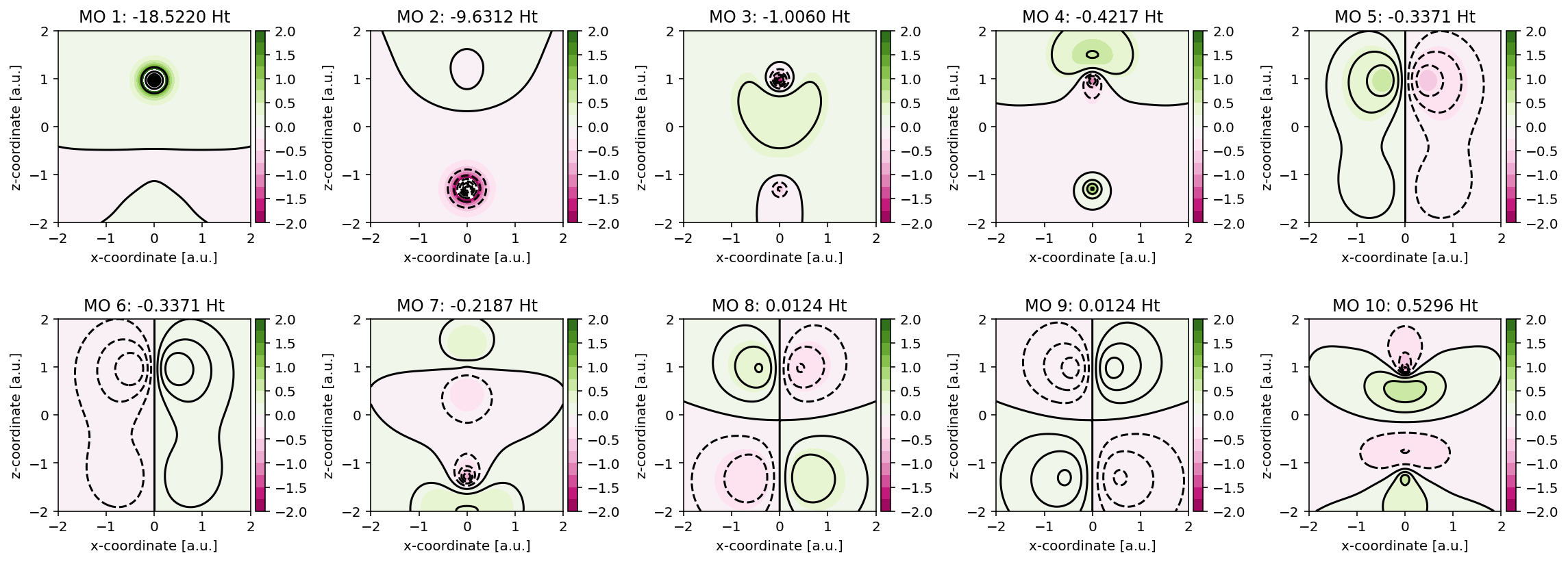
Contour plots for the Kohn-Sham molecular orbitals of CO.

See also

To get a better impression of the three-dimensional shape of the molecular orbitals, it is recommended to produce isosurfaces rather than contour plots.

Isosurfaces

Generating an isosurface is very similar to generating a contour plot, but with the notable difference that the orbital has to be sampled in three-dimensional space. In the script below, an example is provided for one of the \(1\pi\) orbitals of CO. Observe that for generating an isosurface, the algorithm has to be executed twice, once for the positive lobe and once for the negative lobe. The isosurfaces are stored in so-called Polygon File Format files which can be used in your favorite rendering program.

Note

Isosurface generation requires the PyTessel package to be installed. More information can be found here.

import numpy as np
from pydft import MoleculeBuilder, DFT
from pytessel import PyTessel

def main():
    # perform DFT calculation on the CO molecule
    co = MoleculeBuilder().from_name("CO")
    dft = DFT(co, basis='sto3g')
    res = dft.scf(1e-4, verbose=False)
        
    # grab a copy of the MolecularGrid object and of the coefficient matrix
    molgrid = dft.get_molgrid_copy()
    orbc = res['orbc']

    sz = 10     # size of the domain
    npts = 50   # number of sampling points per cartesian direction

    build_isosurface('1pi_pos.ply', molgrid, orbc[:,4], 0.03, sz, npts)
    build_isosurface('1pi_neg.ply', molgrid, orbc[:,4], -0.03, sz, npts)

def build_isosurface(filename, molgrid, coeff, isovalue, sz, npts):
    # produce meshgrid for the unit cell
    x = np.linspace(-sz/2, sz/2, npts)
    zz, yy, xx = np.meshgrid(x, x, x, indexing='ij')
    N = len(x)
    gridpoints = np.zeros((N, N, N, 3))
    gridpoints[:,:,:,0] = xx
    gridpoints[:,:,:,1] = yy
    gridpoints[:,:,:,2] = zz
    gridpoints = gridpoints.reshape((-1,3))

    # build isosurface
    scalarfield = molgrid.get_amplitude_at_points(gridpoints, coeff).reshape(npts, npts, npts)
    unitcell = np.diag(np.ones(3) * sz)

    pytessel = PyTessel()
    vertices, normals, indices = pytessel.marching_cubes(scalarfield.flatten(), scalarfield.shape, unitcell.flatten(), isovalue)
    pytessel.write_ply(filename, vertices, normals, indices)

if __name__ == '__main__':
    main()