Usage
Creating atomic systems
To perform an electronic structure calculation, one first has to define an
atomic system. This can be done in two ways, either manually or by means of the
pypwdft.SystemBuilder class.
Automatic
The most straightforward way is to use the pypwdft.SystemBuilder class.
To build a system, one can run
from pypwdft import SystemBuilder, PeriodicSystem

# create cubic periodic system with lattice size of 10 Bohr units
npts = 16   # number of grid points
sz = 10

# construct CH4 molecule system via SystemBuilder
s = SystemBuilder().from_name('CH4', sz=sz, npts=npts)
To view the unit cell matrix and the atomic coordinates, one can simply invoke
print(s)
which in the above scenario yields the following output
[[10.  0.  0.]
 [ 0. 10.  0.]
 [ 0.  0. 10.]]
6  (5.0000  5.0000  5.0000)
1  (6.1958  6.1958  6.1958)
1  (3.8042  3.8042  6.1958)
1  (3.8042  6.1958  3.8042)
1  (6.1958  3.8042  3.8042)
The following molecules are available via the pypwdft.SystemBuilder
class:
benzene
bf3
ch4
co
ethylene
h2
h2o
he
lih
nh3
Note
Unless otherwise specified, atomic units are used throughout the program. This means that all distances are provided in Bohr units.
Manual
Alternatively, one can also build a system by hand. First, define the unit cell and the number of sampling points per Cartesian direction.
from pypwdft import PeriodicSystem

npts = 32   # number of grid points
sz = 10     # edge size of cubic unit cell
s = PeriodicSystem(sz, npts)
Next, one can add atoms to the PeriodicSystem by means of the
pypwdft.PeriodicSystem.add_atom method
# atomic positions
atompos = np.array([[5.00000000, 5.00000000, 5.00000000],
                    [6.19575624, 6.19575624, 6.19575624],
                    [3.80424376, 3.80424376, 6.19575624],
                    [3.80424376, 6.19575624, 3.80424376],
                    [6.19575624, 3.80424376, 3.80424376]])

# atomic charges
charges = [6, 1, 1, 1, 1] # C + 4 x H

# add atoms to the system
for p,c in zip(atompos, charges):
    s.add_atom(p[0], p[1], p[2], c)
Performing electronic structure calculation
Electronic structure calculations are handled by the pypwdft.PyPWDFT
class. For each separate electronic structure calculation, one creates a fresh
instance of this class. Upon instancing, a pypwdft.PeriodicSystem
instance is provided. Furthermore, the user can select which FFT algorithm is
being used. Three options are available:
NumPy FFT :
numpyScipy FFT :
scipypyFFTW FFT :
pyfftw
By default, pyfftw is used as this algorithm provides the best
performance.
After building the pypwdft.PyPWDFT instance, the electronic structure
calculation can be invoked by running pypwdft.PyPWDFT.scf. This
function allows for several parameters tuning the execution. The default
parameters are however typically suitable. By default, no output is written to
the console, but this can be changed by setting verbose=True. Below,
an example is provided how to set-up a electronic structure calculation.
from pypwdft import PyPWDFT, PeriodicSystem, SystemBuilder

# create cubic periodic system with lattice size of 10 Bohr units
npts = 32   # number of grid points
sz = 10

# construct CH4 molecule system via SystemBuilder
s = SystemBuilder().from_name('CH4', sz=sz, npts=npts)

# construct calculator object
calculator = PyPWDFT(s)

# perform self-consistent field procedure and store results in res object
res = calculator.scf(tol=1e-5, verbose=True)
Upon execution of this code, the following output is written to the console
001 | Etot =  25.72188838 Ht | eps = 2.5722e+01 | dt = 0.5023 s
002 | Etot =  -3.73540233 Ht | eps = 2.9457e+01 | dt = 0.5098 s
003 | Etot = -21.73526459 Ht | eps = 1.8000e+01 | dt = 0.5807 s
...
031 | Etot = -37.74458043 Ht | eps = 2.4958e-05 | dt = 0.9166 s
032 | Etot = -37.74459617 Ht | eps = 1.5732e-05 | dt = 1.0046 s
033 | Etot = -37.74460604 Ht | eps = 9.8741e-06 | dt = 1.0156 s
Furthermore, the result of the calculation are stored in a so-called results dictionary. This dictionary contains the following entries:
Energy: List of total electronic energy per iterationEtot: Total electronic energyEkin: Kinetic energyEnuc: Nuclear attraction energyErep: Electron-electron repulsion energyExc: Exchange-correlation energyedens: Electron density scalar fieldk2: Plane wave vector magnitudesdV: Real-space integration constantEewald: Nuclear-nuclear repulsion (Ewald sum)orbc_fft: Reciprocal-space representation of the molecular orbitalsorbe: Molecular orbital energiesorbc_rs: Real-space representation of the molecular orbitalsttime: Total computation time
Note
All energies are provided in Hartrees.
Visualizing molecular orbitals
Molecular orbitals can be visualized using matplotlib. The results of the pypwdft.PyPWDFT.scf
routine is a dictionary of which one of its elements is orbc_rs. This
element corresponds to a four-dimensional array where the first index loops over
the molecular orbitals with increasing orbital energy.
Two-dimensional projections
By setting the two indices, one can essentially extract a specific z-layer from
the scalar field of any of the molecular orbitals and in turn visualize these
using the imshow function of matplotlib. This is demonstrated in the
script below.
Note
The wave functions generated by a plane wave density functional theory calculation are complex values, i.e.
and as such, it is recommended to visualize both the real and complex parts of the wave function as well as its electron density as given by
# import the required libraries for the test
from pypwdft import PyPWDFT, PeriodicSystem, SystemBuilder
import numpy as np
import matplotlib.pyplot as plt
from mpl_toolkits.axes_grid1 import make_axes_locatable
def main():
# create cubic periodic system with lattice size of 10 Bohr units
npts = 32 # number of grid points
sz = 10
# construct CH4 molecule system via SystemBuilder
s = SystemBuilder().from_name('CH4', sz=sz, npts=npts)
# construct calculator object
calculator = PyPWDFT(s)
# perform self-consistent field procedure and store results in res object
res = calculator.scf(tol=1e-1, verbose=True)
# visualize the occupied molecular orbitals
fig, im = plt.subplots(3,5, dpi=300, figsize=(16,8))
extent=[-sz/2,sz/2,-sz/2,sz/2]
orbe = res['orbe']
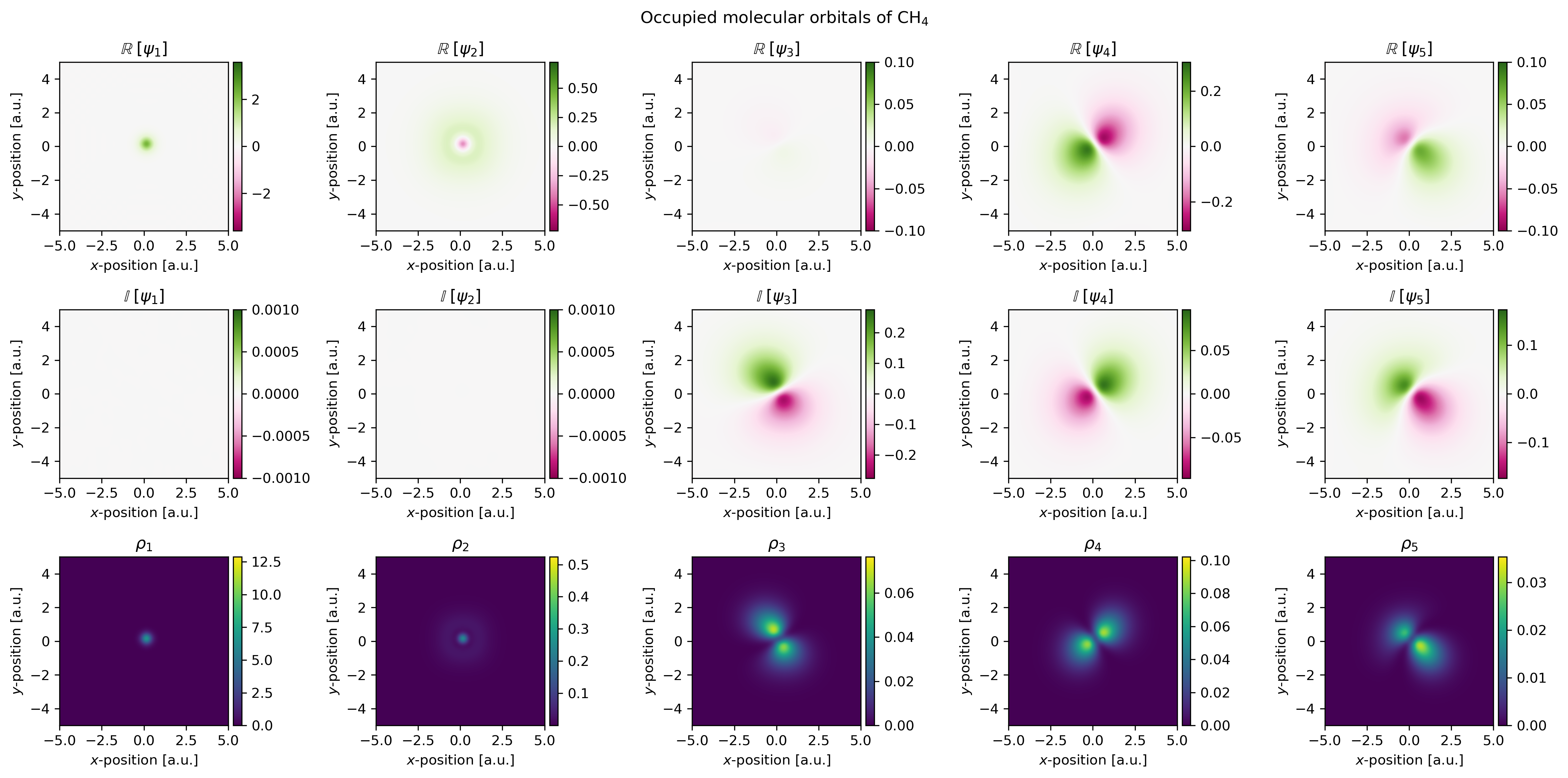
fig.suptitle('Occupied molecular orbitals of CH$_{4}$')
m = np.empty((3,5), dtype=object) # create placeholder for maps
for i in range(0,5):
# visualize the real part of the wave function
field = np.real(res['orbc_rs'][i][npts//2, :, :])
maxval = max(np.max(np.abs(field)), 0.1)
m[0][i] = im[0,i].imshow(field, origin='lower',
interpolation='bicubic', extent=extent, cmap='PiYG',
vmin=-maxval, vmax=maxval)
im[0,i].set_title(r'$\mathbb{R}\;[\psi_{%i}]$' % (i+1))
# visualize the imaginary part of the wave function
field = np.imag(res['orbc_rs'][i][npts//2, :, :])
maxval = max(np.max(np.abs(field)), 0.001)
m[1][i] = im[1,i].imshow(field, origin='lower',
interpolation='bicubic', extent=extent, cmap='PiYG',
vmin=-maxval, vmax=maxval)
im[1,i].set_title(r'$\mathbb{I}\;[\psi_{%i}]$' % (i+1))
# visualize the electron density
m[2][i] = im[2,i].imshow(np.real(res['orbc_rs'][i][npts//2, :, :].conj() *
res['orbc_rs'][i][npts//2, :, :]),
origin='lower', interpolation='bicubic', extent=extent)
im[2,i].set_title(r'$\rho_{%i}$' % (i+1))
for j in range(0,3):
for i in range(0,5):
im[j,i].set_xlabel('$x$-position [a.u.]')
im[j,i].set_ylabel('$y$-position [a.u.]')
divider = make_axes_locatable(im[j,i])
cax = divider.append_axes('right', size='5%', pad=0.05)
fig.colorbar(m[j][i], cax=cax, orientation='vertical')
plt.tight_layout()
if __name__ == '__main__':
main()
The result of running this script is shown below.
Isosurfaces
Alternative to two-dimensional projections, one can also create isosurfaces. For this, we will use the external module PyTessel. For isosurfaces, a relatively large number of sampling points for the scalar fields are required. However, this comes at the expense of computational time. To tackle this, we can use upsampling procedures. Here, we show two such upsampling methods, corresponding to quintic interpolation and frequency-domain upsampling.
Quintic interpolation
We will perform the electronic structure calculation initially using only 32 sampling points per Cartesian direction and follow up using quintic interpolation to “upsample” the scalar fields. An example of this process is shown in the image below.
import numpy as np
from pytessel import PyTessel
from scipy.interpolate import RegularGridInterpolator
from pypwdft import PyPWDFT, SystemBuilder, PeriodicSystem

def main():
    # create cubic periodic system with lattice size of 10 Bohr units
    npts = 32       # number of grid points
    sz = 10

    # construct CO molecule system via SystemBuilder
    s = SystemBuilder().from_name('CO', sz=sz, npts=npts)

    # construct calculator object
    calculator = PyPWDFT(s)

    # perform self-consistent field procedure and store results in res object
    res = calculator.scf(tol=1e-5, nsol=9, verbose=True)

    # generate PyTessel object
    pytessel = PyTessel()

    for i in range(2,9):
        print('Building isosurfaces: %02i' % (i+1))
        scalarfield = interpolate_grid(res['orbc_rs'][i], sz, npts, 4)
        unitcell = np.identity(3) * sz

        # build positive real isosurface
        vertices, normals, indices = pytessel.marching_cubes(scalarfield.real.flatten(), scalarfield.shape, unitcell.flatten(), 0.1)
        pytessel.write_ply('MO_PR_%02i.ply' % (i+1), vertices, normals, indices)

        # build negative real isosurface
        vertices, normals, indices = pytessel.marching_cubes(scalarfield.real.flatten(), scalarfield.shape, unitcell.flatten(), -0.1)
        pytessel.write_ply('MO_NR_%02i.ply' % (i+1), vertices, normals, indices)

        # build positive imaginary isosurface
        vertices, normals, indices = pytessel.marching_cubes(scalarfield.imag.flatten(), scalarfield.shape, unitcell.flatten(), 0.1)
        pytessel.write_ply('MO_PI_%02i.ply' % (i+1), vertices, normals, indices)

        # build negative imaginary isosurface
        vertices, normals, indices = pytessel.marching_cubes(scalarfield.imag.flatten(), scalarfield.shape, unitcell.flatten(), -0.1)
        pytessel.write_ply('MO_NI_%02i.ply' % (i+1), vertices, normals, indices)

def interpolate_grid(scalarfield, sz, npts, amp=2):
    x = np.linspace(0, sz, npts)
    interp = RegularGridInterpolator((x,x,x), scalarfield, method='quintic')
    s = PeriodicSystem(sz, npts * amp)
    points = s.get_r()

    return interp(points)

if __name__ == '__main__':
    main()
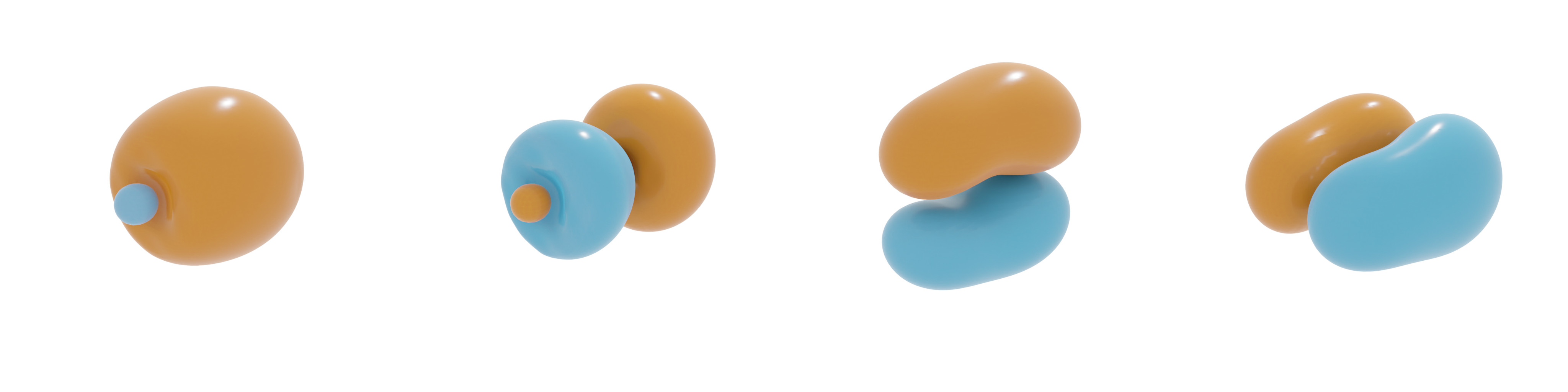
In the image below, the isosurfaces corresponding to the real part of the scalar field for the 3σ, 4σ and 1π orbitals are visualized.
Frequency domain upsampling
In the code below, an example for frequency scale upsampling is shown.
import numpy as np
from pytessel import PyTessel
from pypwdft import PyPWDFT, SystemBuilder

def main():
    # create cubic periodic system with lattice size of 10 Bohr units
    npts = 32       # number of grid points
    sz = 10

    # construct CO molecule system via SystemBuilder
    s = SystemBuilder().from_name('CH4', sz=sz, npts=npts)

    # construct calculator object
    calculator = PyPWDFT(s)

    # perform self-consistent field procedure and store results in res object
    res = calculator.scf(tol=1e-5, verbose=True)

    # print molecular orbital energies
    print(res['orbe'])

    # generate PyTessel object
    pytessel = PyTessel()

    for i in range(5):
        print('Building isosurfaces: %02i' % (i+1))
        scalarfield = upsample_grid(res['orbc_fft'][i], sz**3, 4)
        unitcell = np.identity(3) * sz

        # build positive real isosurface
        vertices, normals, indices = pytessel.marching_cubes(scalarfield.real.flatten(), scalarfield.shape, unitcell.flatten(), 0.03)
        pytessel.write_ply('MO_PR_%02i.ply' % (i+1), vertices, normals, indices)

        # build negative real isosurface
        vertices, normals, indices = pytessel.marching_cubes(scalarfield.real.flatten(), scalarfield.shape, unitcell.flatten(), -0.03)
        pytessel.write_ply('MO_NR_%02i.ply' % (i+1), vertices, normals, indices)

        # build positive imaginary isosurface
        vertices, normals, indices = pytessel.marching_cubes(scalarfield.imag.flatten(), scalarfield.shape, unitcell.flatten(), 0.03)
        pytessel.write_ply('MO_PI_%02i.ply' % (i+1), vertices, normals, indices)

        # build negative imaginary isosurface
        vertices, normals, indices = pytessel.marching_cubes(scalarfield.imag.flatten(), scalarfield.shape, unitcell.flatten(), -0.03)
        pytessel.write_ply('MO_NI_%02i.ply' % (i+1), vertices, normals, indices)

def upsample_grid(scalarfield_fft, Omega, upsample=4):
    Nx, Ny, Nz = scalarfield_fft.shape
    Nx_up = Nx * upsample
    Ny_up = Nx * upsample
    Nz_up = Nx * upsample

    # shift the frequencies
    fft = np.fft.fftshift(scalarfield_fft)

    # perform padding
    fft_upsampled = np.pad(fft, [((Nz_up-Nz)//2,),
                                ((Ny_up-Ny)//2,),
                                ((Nx_up-Nx)//2,)], 'constant')

    # shift back
    fft_hires = np.fft.ifftshift(fft_upsampled)

    return np.fft.ifftn(fft_hires) * np.prod([Nx_up, Ny_up, Nz_up]) / np.sqrt(Omega)

if __name__ == '__main__':
    main()
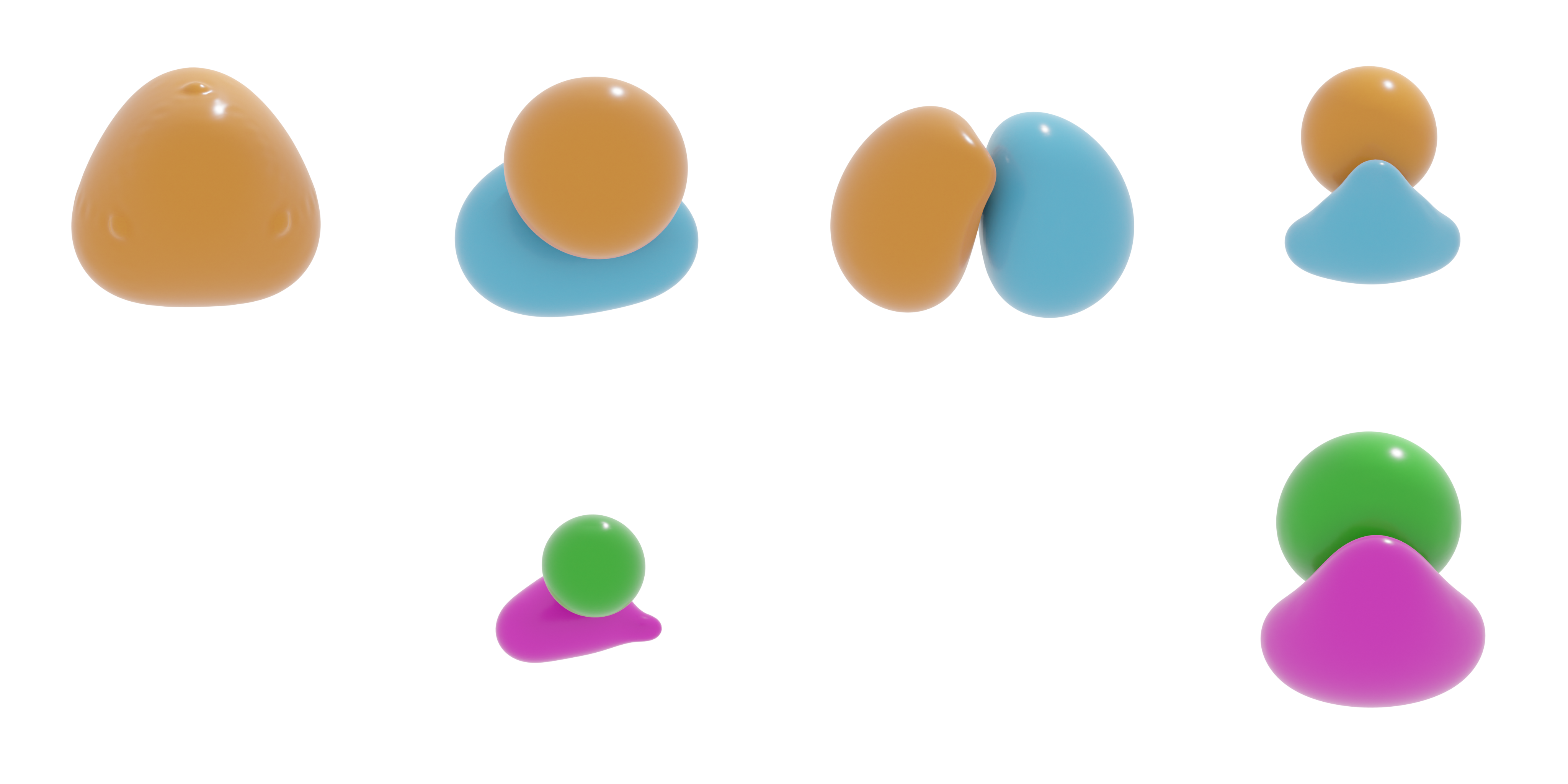
Using the above scripts, the molecular orbitals as shown in the image below are found. Here, an isovalue of 0.03 was used. Since the molecular orbitals are complex-valued, both the real-part (orange-blue) as well as the the imaginary part (purple-green) is visualized provided that the imaginary part has a significant contribution. Though it might not look to be the case based on the shape of the orbitals, if one runs the above script, it can be verified that the latter three orbitals have equal orbital energies.