Tutorials

Converting OUTCAR to YAML file

This tutorial explains how one can parse a single VASP frequency calculation and constructs a single .yaml-based data entry from this calculation.

Prerequisites

First, we need to prepare an OUTCAR file that we wish to parse. Several example OUTCAR are stored in tests/data which we can unpack. For this tutorial, we assume that we are working under examples/individual.

Go to this folder

cd examples/individual

and run

unzip ../../tests/data/OUTCAR_Ru1121_CH.zip

This should give the following output:

Archive:  ../../tests/data/OUTCAR_Ru1121_CH.zip
   inflating: OUTCAR_Ru1121_CH

Building YAML files

The OUTCAR_Ru1121_CH file contains a frequency calculation of a CH molecule adsorbed on a Ru(11-21) surface. To build the yaml file, we run

pymkmkit freq2yaml OUTCAR_Ru1121_CH -o ru1121_c.yaml --average-pairs

The option --average-pairs is needed in this case because the OUTCAR file contains a metallic slab on which CH has been adsorbed on both sides. Thus, when sampling the frequencies for a single CH adsorbate, we need to average out the frequencies of both the top and bottom CH fragment.

Note

The --average-pairs option is required for some older slab calculations. Historically, adsorbates were placed on both sides of a metal slab to cancel dipole moments before dipole corrections became standard in VASP. Modern calculations typically use dipole corrections instead and only place the adsorbate on one side.

In these legacy setups, two identical adsorbates (top and bottom) produce duplicate vibrational modes. Because frequencies are computed using a finite-difference approach, small numerical differences appear between the paired modes. Averaging the pairs recovers the vibrational frequencies corresponding to a single adsorbate while reducing numerical noise.

Tip

To visualize the frequency calculation and inspect vibrational modes, you can use Atom Architect. Visualizing the displacements can help identify paired modes and confirm the averaging.

Understanding the generated YAML file

The generated YAML file stores all information required to reproduce and reuse the thermodynamic state in a microkinetic model.

Below we highlight the key sections and why they are stored.

`pymkmkit`

Metadata describing how the file was created.

pymkmkit:
  version: 0.1.0
  generated: 2026-02-26T07:21:02Z

Field	Purpose
`version`	pymkmkit version used to generate the file
`generated`	Timestamp for provenance and reproducibility

This metadata ensures traceability and helps diagnose differences between datasets.

`structure`

Describes the atomic structure used in the calculation.

structure:
  formula: Ru48C2H2
  lattice_vectors: [...]
  coordinates_direct: [...]
  pbc: [true, true, true]

Field	Purpose
`formula` / `n_atoms`	Quick identification of system composition and size
`lattice_vectors`	Defines the periodic simulation cell
`coordinates_direct`	Atomic positions in fractional coordinates
`pbc`	Periodic boundary conditions

Storing the full structure allows the system to be reconstructed and verified.

`calculation`

Records how the calculation was performed.

calculation:
  code: VASP
  type: frequency
  incar: {...}
  potcar:
    - PAW_PBE Ru
    - PAW_PBE C
    - PAW_PBE H

Field	Purpose
`code` / `type`	Simulation software and calculation type
`incar`	Important settings affecting accuracy and results
`potcar`	Pseudopotentials used

These parameters are essential for reproducibility and validation.

`energy`

energy:
  electronic: -433.134185

The electronic energy forms the basis for adsorption energies, reaction energies, and activation barriers.

`vibrations`

Contains vibrational data required to compute thermodynamic properties.

vibrations:
  frequencies_cm-1:
    - 2886.2
    - 714.1
  partial_hessian:
    dof_labels:
      - 49X
      - 49Y
      - 49Z
      - 50X
      - 50Y
      - 50Z
      - 51X
      - 51Y
      - 51Z
      - 52X
      - 52Y
      - 52Z
    matrix: [...]
  paired_modes_averaged: true

Field	Purpose
`frequencies_cm-1`	Vibrational modes used in partition functions
`partial_hessian`	Hessian submatrix for adsorbate degrees of freedom (stored for reuse)
`partial_hessian.dof_labels`	Maps each Hessian row/column to an atom index and Cartesian direction (e.g. `49X`), i.e., which coordinates were displaced in the finite-difference frequency calculation
`paired_modes_averaged`	Indicates symmetric slab modes were averaged

Vibrational data enable computation of:

zero-point energies
entropy and heat capacity
pre-exponential factors in rate constants

The dof_labels make the partial Hessian interpretable: they encode exactly which atoms were perturbed and in which Cartesian direction when constructing the finite-difference Hessian, so the stored matrix can be validated, visualized, or reprocessed later.

Tip

YAML files generated by pymkmkit can be visualized using Atom Architect. The program can display structures, vibrational modes, and displaced coordinates, making it easier to inspect the finite-difference perturbations and verify the results.

Building `network.yaml` file

This section explains how to build a reaction network file, using examples/Ru1121/network.yaml as an example.

The file has four key sections:

stable_states
transition_states
network (elementary reaction steps)
paths (named combinations of elementary reaction steps)

Stable and transition states

The first two set of entries in the yaml file correspond to the stable_states and transition_states. The names are self-explanatory. Both sections are lists of YAML references. Each entry defines:

name: shorthand (unique) label used later in step definitions
file: relative path to the corresponding state YAML file

Examples

For example, in examples/Ru1121/network.yaml we find:

stable_states:
  - name: CO*
    file: ISFS/co.yaml
  - name: C*
    file: ISFS/c.yaml

transition_states:
  - name: CO_diss
    file: TS/co_diss.yaml

This defines two stable states, corresponding to CO* and C* adsorbed on the catalytic surface whose state is defined by the YAML files ISFS/co.yaml and TS/co_diss.yaml, respectively.

Defining elementary reaction steps

The network section is a list of elementary steps. Each step has:

name: unique step identifier
type: surf or ads
reaction: human-readable reaction string

For surf steps, energies are given through forward and backward blocks, each containing:

ts: list of transition-state terms
is: list of initial-state terms
normalization: divisor used to normalize to one adsorbate/site unit

Each ts or is term has:

name: label from stable_states or transition_states
stoichiometry: multiplicative factor

For ads steps, the file uses is and fs (initial/final state) plus normalization.

The normalization entry is used when calculations contain multiple symmetry-equivalent adsorbates (e.g., adsorbates on both slab faces). Since the computed energies and ZPE contributions correspond to the combined system, normalization: 2 converts them to per-adsorbate values.

How pymkmkit evaluates barriers (including ZPE)

For a surface step direction (forward or backward), pymkmkit computes:

\[\Delta E^{\ddagger}_{\mathrm{elec}} = \frac{\sum_i \nu_i E_{\mathrm{elec}}(\mathrm{TS}_i) - \sum_j \nu_j E_{\mathrm{elec}}(\mathrm{IS}_j)}{N_{\mathrm{norm}}}\]

\[\Delta E^{\ddagger}_{\mathrm{zpe}} = \sum_i \nu_i E_{\mathrm{zpe}}(\mathrm{TS}_i) - \sum_j \nu_j E_{\mathrm{zpe}}(\mathrm{IS}_j)\]

\[\Delta E^{\ddagger}_{\mathrm{tot}} = \Delta E^{\ddagger}_{\mathrm{elec}} + \Delta E^{\ddagger}_{\mathrm{zpe}}\]

with

\[E_{\mathrm{zpe}} = \frac{1}{2} \sum_k h \nu_k\]

implemented from vibrational frequencies in cm^-1 as

\[E_{\mathrm{zpe}}\,\mathrm{(eV)} = \frac{1}{2}\sum_k \nu_k\,\times\,1.239841984\times10^{-4}\]

Examples

CO dissociation

- name: CO dissociation
  type: surf
  reaction: CO* + * => C* + O*
  forward:
    ts:
      - name: CO_diss
        stoichiometry: 1
    is:
      - name: CO*
        stoichiometry: 1
    normalization: 2

Forward barrier equations are:

\[\Delta E^{\ddagger}_{\mathrm{elec,fwd}} = \frac{E_{\mathrm{elec}}(\mathrm{CO\_diss}) - E_{\mathrm{elec}}(\mathrm{CO^*})} {2}\]

\[\Delta E^{\ddagger}_{\mathrm{zpe,fwd}} = E_{\mathrm{zpe}}(\mathrm{CO\_diss}) - E_{\mathrm{zpe}}(\mathrm{CO^*})\]

\[\Delta E^{\ddagger}_{\mathrm{tot,fwd}} = \Delta E^{\ddagger}_{\mathrm{elec,fwd}} + \Delta E^{\ddagger}_{\mathrm{zpe,fwd}}\]

C hydrogenation

- name: C hydrogenation
  type: surf
  reaction: C* + H* => CH* + *
  forward:
    ts:
      - name: C_hydr
        stoichiometry: 1
      - name: empty
        stoichiometry: 1
    is:
      - name: C*
        stoichiometry: 1
      - name: H*
        stoichiometry: 1
    normalization: 2

Forward barrier equations are:

\[\Delta E^{\ddagger}_{\mathrm{elec,fwd}} = \frac{ E_{\mathrm{elec}}(\mathrm{C\_hydr}) + E_{\mathrm{elec}}(\mathrm{empty}) - E_{\mathrm{elec}}(\mathrm{C^*}) - E_{\mathrm{elec}}(\mathrm{H^*}) } {2}\]

\[\Delta E^{\ddagger}_{\mathrm{zpe,fwd}} = E_{\mathrm{zpe}}(\mathrm{C\_hydr}) + E_{\mathrm{zpe}}(\mathrm{empty}) - E_{\mathrm{zpe}}(\mathrm{C^*}) - E_{\mathrm{zpe}}(\mathrm{H^*})\]

\[\Delta E^{\ddagger}_{\mathrm{tot,fwd}} = \Delta E^{\ddagger}_{\mathrm{elec,fwd}} + \Delta E^{\ddagger}_{\mathrm{zpe,fwd}}\]

Grouping elementary steps into mechanisms using paths

The paths section defines named sequences of network steps, for example to evaluate overall reaction energies or to build potential energy diagrams.

Each path contains:

name: path identifier
startlabel: label shown for the initial state in PED output
steps: ordered list of elementary steps by name

Optional per-step entries:

factor (default 1): multiply that step contribution; this is used to represent successive applications of this elementary reaction step, for example when you want sixfold 1/2 H2 adsorption.
label: custom state label for PED annotations

Example (from the Ru(11-21) case):

paths:
  - name: methanation
    startlabel: CO + 3H2
    steps:
      - name: CO adsorption
        label: CO* + 3H2
      - name: H2 adsorption
        factor: 6
        label: CO* + 6H*

Evaluating network files

From the repository root, you can run:

pymkmkit read_network examples/Ru1121/network.yaml

This parses all states and prints step-wise quantities:

for surf steps: forward and reverse barriers (including ZPE correction)
for ads steps: adsorption heat (including ZPE correction)

which yields the following output:

Reaction: CO* + * => C* + O*
  Forward barrier: 0.708003 eV (inc. ZPE-corr: -0.031787)
  Reverse barrier: 0.743850 eV (inc. ZPE-corr: -0.024853)
Reaction: C* + H* => CH* + *
  Forward barrier: 0.406754 eV (inc. ZPE-corr: -0.047930)
  Reverse barrier: 0.267382 eV (inc. ZPE-corr: -0.139948)
Reaction: CH* + H* => CH2* + *
  Forward barrier: 0.703780 eV (inc. ZPE-corr: -0.038874)
  Reverse barrier: 0.362366 eV (inc. ZPE-corr: -0.108891)
Reaction: CH2* + H* => CH3* + *
  Forward barrier: 0.672479 eV (inc. ZPE-corr: 0.046713)
  Reverse barrier: 0.657561 eV (inc. ZPE-corr: -0.122669)
Reaction: CH3* + H* => CH4 + 2*
  Forward barrier: 1.198466 eV (inc. ZPE-corr: -0.012794)
  Reverse barrier: 0.466999 eV (inc. ZPE-corr: -0.138733)
Reaction: O* + H* => OH* + *
  Forward barrier: 0.925349 eV (inc. ZPE-corr: -0.075468)
  Reverse barrier: 0.607454 eV (inc. ZPE-corr: -0.197065)
Reaction: OH* + H* => H2O* + *
  Forward barrier: 1.102802 eV (inc. ZPE-corr: 0.048977)
  Reverse barrier: 0.446876 eV (inc. ZPE-corr: -0.068496)
Reaction: CO + * => CO*
  Adsorption heat: -1.638042 eV (inc. ZPE-corr: 0.021169)
Reaction: H2 + 2* => 2H*
  Adsorption heat: -0.585109 eV (inc. ZPE-corr: 0.030218)
Reaction: H2O + * => H2O*
  Adsorption heat: -0.643202 eV (inc. ZPE-corr: 0.059390)

To evaluate total energies of all named paths:

pymkmkit evaluate_paths examples/Ru1121/network.yaml

This sums the (factor-weighted) step reaction heats for each path as given by the following output:

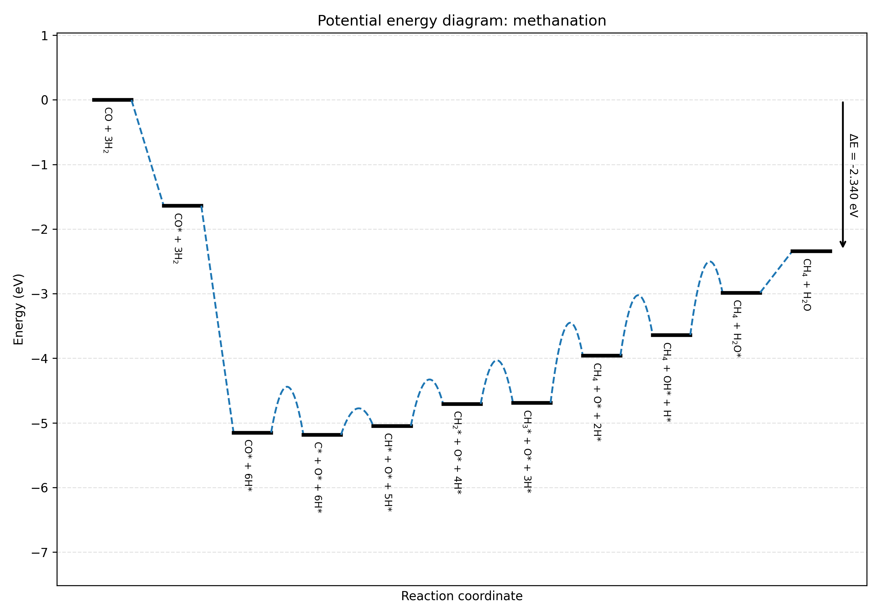
Path methanation: -2.340352 eV

To construct a potential energy diagram for one path:

pymkmkit build_ped examples/Ru1121/network.yaml methanation methanation.png

This builds the PED of the methanation path and writes it to methanation.png.

Tutorials

Converting OUTCAR to YAML file

Prerequisites

Building YAML files

Understanding the generated YAML file

pymkmkit

structure

calculation

energy

vibrations

Building network.yaml file

Stable and transition states

Examples

Defining elementary reaction steps

How pymkmkit evaluates barriers (including ZPE)

Examples

Grouping elementary steps into mechanisms using paths

Evaluating network files

`pymkmkit`

`structure`

`calculation`

`energy`

`vibrations`

Building `network.yaml` file