Tutorials
Important
We assume you have a working environment for running the C++ and Python scripts. If not, head over to the Getting Started section.
For all commands and instructions shown below, unless explicitly stated, we assume that these are executed from the root folder of the repository.
Make sure an
outputfolder is present in the repository root. Graphs will be written in that folder.
Tutorial: Creating a neural network for methane
Dataset construction and network training
In this tutorial, we are going to draft a Behler-Parrinello Neural Network for
the methane molecule. To build and train the network, we require a dataset. This
dataset is obtained by running AIMD calculations in VASP. The result of this
AIMD simulation is (1) a XDATCAR file. For each entry in the
XDATCAR we need to associate an energy value, which can be obtained
from the OUTCAR file using the following one-liner:
grep "y w" OUTCAR | awk '{print $7}' > XDATEN
The XDATCAR and the freshly created XDATEN are both
human-readable files. For efficient (fast!) data handling, we are going to
convert these to a custom binary pkg file. This is done using one of the
Python scripts as found in the pysrc folder.
For convenience purposes, example XDATCAR and XDATEN files for
both a low- and high-temperature AIMD run are already available in the
/data folder, which we are going to conver to .pkg files using the
commands as seen below:
python3 pysrc/xdatcar2pack.py -x data/XDATCAR_ch4_lt -e data/XDATEN_ch4_lt -o data/ch4_lt.pkg
python3 pysrc/xdatcar2pack.py -x data/XDATCAR_ch4_ht -e data/XDATEN_ch4_ht -o data/ch4_ht.pkg
The output of either of these commands should look something like this:
100%|█████████████████████████████████████████████████████████████████████████████████████████| 10000/10000 [00:00<00:00, 25896.52it/s]
Stored 10000 data files in data/ch4_lt.pkg
These commands will generate two new files:
data/ch4_lt.pkgdata/ch4_ht.pkg
These files contain the geometry and the energies for a number of structures, in our specific case, 10,000 per file.
Next, we need to generate the Behler-Parrinello symmetry function coefficients
for all these structures. This is a relatively time-consuming step and for that
reason, this generation process is done using a custom C++ program, called
BPSFP.
./build/bpsfp -d data/ch4_lt.pkg -r data/request -o data/ch4_lt_coeff.npz
./build/bpsfp -d data/ch4_ht.pkg -r data/request -o data/ch4_ht_coeff.npz
The output of either of these commands should look something like this:
Progress: [==================================================] 100%
All done!
These commands will create two more files:
data/ch4_lt_coeff.pkgdata/ch4_ht_coeff.pkg
At this stage, we are done generating the dataset and we can now use this
dataset to train our network. For this fitting step (executed via
torch/train_ch4.py), we use the local perceptronium Python
package that ships with this repository. The package is primarily focused on
building the neural-network inputs (dataset handling, request-file parsing,
and symmetry-function descriptor preparation), while still providing lightweight
utilities for model definition, training, plotting, and model export.
In other words, perceptronium is provided as a simple utility package for this tutorial: it demonstrates one complete fitting workflow and also shows how to consume the resulting network description for downstream tasks (for example, optimization scripts that load the trained model).
The default architecture used in this tutorial is defined in
torch/perceptronium/network.py via netconfig=[124, 64, 16, 1].
Each atom is processed by a type-specific sub-network with fully connected
layers (124 input features from Behler-Parrinello descriptors, followed by
hidden layers of 64 and 16 neurons, and a scalar output). ReLU activations are
applied between hidden layers, and the final layer remains linear to produce an
atomic embedding energy. During the molecular forward pass, the package applies
the sub-network matching each atom type and sums all per-atom energies to
obtain the total system energy. A visual representation of this per-atom
network is provided below.

To construct and train the BPNN, the Python script as shown below is used. During training, only the parameters specific to each atom type are optimized. This means that while five atomic neural networks are used to compute the system energy, four of them—corresponding to hydrogen (H) share the same network parameters.
You can copy the Python below and execute it, but a copy of it is placed under
/torch.
import os
from perceptronium import MultiMolDataset, MultiMolNet, MolFitter

ROOT = os.path.dirname(__file__)

def main():
    paths = [
        os.path.join(ROOT, '..', 'data', 'ch4_ht_coeff.npz'),
    ]
    dataset = MultiMolDataset(paths, os.path.join(ROOT, '..', 'data', 'request'))

    outpath = os.path.join(ROOT, '..', 'output')
    os.makedirs(outpath, exist_ok=True) # ensure folder is created if it does not yet exists

    # set-up fitter class and start training the network
    fitter = MolFitter(num_types=2)
    fitter.fit(dataset, num_epochs=2000)

    # produce fitting plots
    fitter.create_parity_plot(graphfile=os.path.join(outpath, 'ch4_parity.png'))
    fitter.create_loss_history_plot(graphfile=os.path.join(outpath, 'ch4_loss_history.png'))

    # store network
    fitter.save_model(os.path.join(outpath, 'ch4_network.pth'))

if __name__ == '__main__':
    main()
After running the Python script via
cd torch
python train_ch4.py
We should see an output similar to this:
CUDA Available: True
Number of GPUs: 1
GPU Name: NVIDIA GeForce RTX 5090
Using device: cuda
Epoch     Train Loss     Val Loss       Time (sec)
==================================================
    1     129.963365      40.432288      0.82
    2      29.190743      21.992233      0.26
    3      18.683928      13.131295      0.26
    4      10.017776       6.383904      0.20
    5       4.363754       2.401630      0.21
    6       1.652315       0.979695      0.22
    7       0.781263       0.587972      0.21
    8       0.548366       0.469764      0.26
    9       0.465530       0.429274      0.25
    10       0.433574       0.410703      0.23

...

    1995       0.032276       0.043959      0.22
    1996       0.033596       0.039676      0.22
    1997       0.033915       0.041398      0.20
    1998       0.038798       0.043789      0.22
    1999       0.032037       0.049397      0.27
    2000       0.036683       0.042168      0.25
Tip
If you are running your optimization on a GPU (you should, it is faster!),
you can check upon its usage via watch nvidia-smi, which displays
something akin to:
+-----------------------------------------------------------------------------------------+
| NVIDIA-SMI 580.102.01             Driver Version: 581.57         CUDA Version: 13.0     |
+-----------------------------------------+------------------------+----------------------+
| GPU  Name                 Persistence-M | Bus-Id          Disp.A | Volatile Uncorr. ECC |
| Fan  Temp   Perf          Pwr:Usage/Cap |           Memory-Usage | GPU-Util  Compute M. |
|                                         |                        |               MIG M. |
|=========================================+========================+======================|
|   0  NVIDIA GeForce RTX 5090        On  |   00000000:01:00.0  On |                  N/A |
| 50%   32C    P0             91W /  575W |    3879MiB /  32607MiB |     10%      Default |
|                                         |                        |                  N/A |
+-----------------------------------------+------------------------+----------------------+
The watch part ensures this screen is updated every 2 seconds.
After completion of the Python script as shown above, two files are produced
in /output:
/output/ch4_parity.png/output/ch4_loss_history.png
We discuss the results displayed in these files in more detail below.
Training results and interpretation
Note
The results presented here should be considered as representative and the actual results you will obtain in your own simulation(s) might differ slightly.
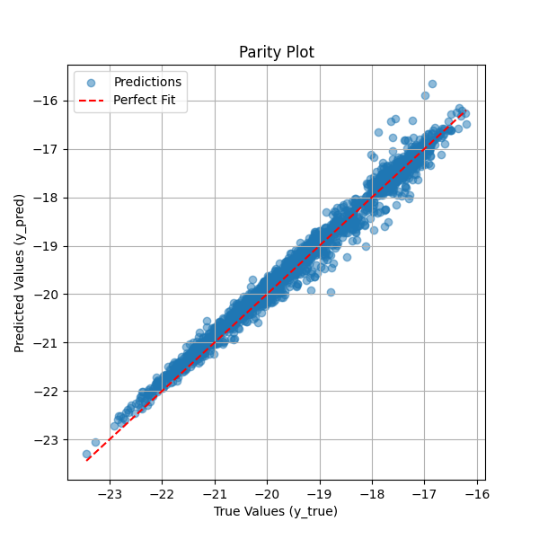
The parity plot below compares the predicted total system energy against the true system energy. Each blue point represents a single prediction, while the red dashed line indicates the ideal scenario where predicted values perfectly match the true values. The close alignment of most points along this diagonal suggests that the neural network effectively learns to sum the per-atom embedding energies to produce accurate system energy estimates. Some deviations at higher energy values indicate minor prediction errors, but overall, the model demonstrates strong performance in capturing the relationship between atomic environments and total system energy. This visualization serves as a key diagnostic tool for assessing the accuracy of the trained neural network.
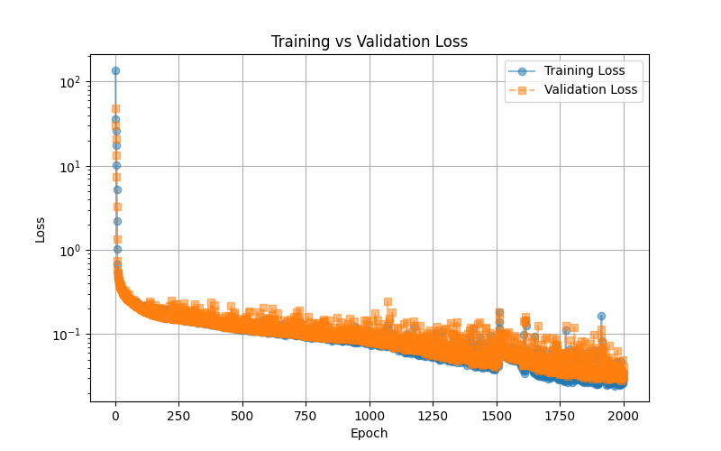
The training vs. validation loss plot illustrates the model’s learning progress over 2000 epochs. The blue line represents the training loss, while the orange dashed line represents the validation loss. Initially, both losses start high, rapidly decreasing as the model learns to minimize error. Over time, the loss continues to decline smoothly, indicating stable training. The close alignment between training and validation loss suggests that the model generalizes well without significant overfitting. Some fluctuations in validation loss are expected due to variations in the validation set, but overall, the trend indicates that the neural network successfully optimizes its parameters to predict total system energy accurately. This plot serves as an essential tool for diagnosing training stability and model performance.
Network utilization: geometry optimizaton of methane
This script demonstrates how to optimize the geometry of a methane (CH₄) molecule using a neural network trained to predict atomic energies. The optimization is performed using the Nelder-Mead algorithm, which iteratively adjusts atomic positions to minimize the predicted energy of the system. At each step, the neural network evaluates the energy based on symmetry function descriptors, and the lowest-energy configuration is tracked. The script provides a practical example of using machine learning to refine molecular structures without requiring explicit force calculations.
Additionally, the script saves the optimization trajectory as an animated GIF, allowing users to visually inspect how the methane molecule’s structure evolves over time. This is particularly useful for analyzing the convergence behavior and ensuring that the optimization leads to a physically meaningful configuration.
import os
import time
import numpy as np
import ase.io
from ase import Atoms
from ase.visualize import view
from ase.data import atomic_numbers
import torch
from scipy.optimize import minimize
from perceptronium import SymmetryFunctionCalculator

# Define the root directory
ROOT = os.path.dirname(__file__)

def main():
    """
    Main function to optimize methane molecule geometry using a trained neural network.
    """
    # Define atomic symbols and initial positions for methane (CH4)
    symbols = ['C', 'H', 'H', 'H', 'H']
    positions = np.array([
        [5.0, 5.0, 5.0],
        [6.0, 5.0, 5.0],
        [4.0, 5.0, 5.0],
        [5.0, 6.0, 5.0],
        [5.0, 4.0, 5.0]
    ])

    # Create an ASE Atoms object (no periodic boundary conditions)
    methane = Atoms(symbols=symbols, positions=positions)
    methane.center(vacuum = 0.0)
    methane.rotate(45, 'z')

    # Initialize Symmetry Function Calculator
    sfc = SymmetryFunctionCalculator(os.path.join(ROOT, '..', 'data', 'request'),
                                    [atomic_numbers[element] for element in ['C', 'H']])

    # Load trained neural network model
    device = torch.device("cuda" if torch.cuda.is_available() else "cpu")
    torch.set_float32_matmul_precision('high')
    mask = torch.tensor(np.ones(len(methane))).to(device)
    model_path = os.path.join(ROOT, '..', 'output', 'ch4_network.pth')
    model = torch.load(model_path, weights_only=False)
    model.to(device).eval()
    model = torch.compile(model)

    # Track iteration history
    iteration_data = []  # Store energy and time per iteration
    position_data = []    # Store molecular positions per iteration
    start_time = time.time()  # Start timer
    bestenergy = float('inf')  # Initialize best energy as a large value
    energy = 0  # Initialize energy value

    def calculate_energy(pos):
        """
        Compute the energy of the system given atomic positions.
        """
        nonlocal energy

        # Compute symmetry function coefficients
        coeff = sfc.calculate(pos.reshape((len(methane), -1)), methane.get_atomic_numbers())
        input_tensor = torch.tensor(coeff, dtype=torch.float32).unsqueeze(0).to(device)

        # Perform inference with the trained model
        with torch.no_grad():
            energy = model(input_tensor, mask=mask).cpu().detach().numpy()[0, 0]
        return energy

    def callback(current_positions):
        """
        Callback function to track optimization progress.
        """
        nonlocal start_time, bestenergy, energy

        # Update best energy if improved
        if energy < bestenergy:
            bestenergy = energy
            position_data.append(current_positions.reshape((len(methane), -1)))

            # Compute elapsed time
            elapsed_time = time.time() - start_time
            start_time = time.time()  # Reset timer for next iteration

            # Store iteration data
            iteration_data.append((len(iteration_data) + 1, energy, elapsed_time))

            # Print iteration progress
            print(f"Iteration {len(iteration_data)}: Energy = {energy:.6f}, Time = {elapsed_time:.4f} sec")

    # Optimize molecular geometry using Nelder-Mead (Simplex Search)
    result = minimize(
        fun=calculate_energy,                       # Energy function
        x0=positions.flatten(),                     # Flattened initial positions
        method='Nelder-Mead',                       # Gradient-free optimization
        callback=callback,                          # Track iterations
        options={'maxiter': 5000, 'fatol': 1e-4}    # Stopping criteria
    )

    # Store optimized atomic configurations, add a unitcell mainly for
    # visualization purposes
    atoms_list = [Atoms(symbols=symbols, positions=pos) for pos in position_data]
    for atoms in atoms_list:
        atoms.set_cell([5.0, 5.0, 5.0])
        atoms.center()

    # store as animated gif
    ase.io.write(os.path.join(ROOT, '..', 'output', 'ch4opt.gif'), atoms_list, format='gif', interval=100, rotation='-90x')

if __name__ == '__main__':
    main()
Optimization results for methane
The animated GIF illustrates the optimization process of a methane (CH₄) molecule, starting from an intentionally unfavorable geometry. The script automatically refines the atomic positions by minimizing the predicted energy using a neural network model. However, since the dataset used to train the model does not contain the optimal methane geometry, the predicted energy is an extrapolation rather than an exact value. Despite this limitation, the final structure seem to align well with the expected tetrahedral geometry of methane, yet merely using a visual representation can be misleading, as we are about to show.

Using the following small snippet, we can also plot the C-H bond lengths as function of the evolution steps
def visualize_bond_lengths(atoms_list):
"""
Visualizes C-H bond lengths for each Atoms object in the trajectory.
Returns a dictionary with lists of bond lengths over time.
"""
bond_data = {f"H{i+1}": [] for i in range(4)}  # Store bond lengths for each H

for atoms in atoms_list:
    c_index = 0  # Assuming the first atom (index 0) is Carbon
    h_indices = [1, 2, 3, 4]  # Hydrogen indices

    # Compute bond lengths for this step
    bond_lengths = [atoms.get_distance(c_index, h) for h in h_indices]

    # Store in respective lists
    for i, length in enumerate(bond_lengths):
        bond_data[f"H{i+1}"].append(length)

# Generate time steps (assuming frames are indexed sequentially)
time_steps = list(range(len(atoms_list)))

# Plot the evolution of each C-H bond length over time
plt.figure(figsize=(8, 5))
for h_label, bond_lengths in bond_data.items():
    plt.plot(time_steps, bond_lengths, label=h_label, marker='o', alpha=0.5)

plt.xlabel("Time Step")
plt.ylabel("C-H Bond Length (Å)")
plt.title("Evolution of C-H Bond Lengths in Methane")
plt.legend()
plt.grid(True)
plt.show()
which yields the following graph
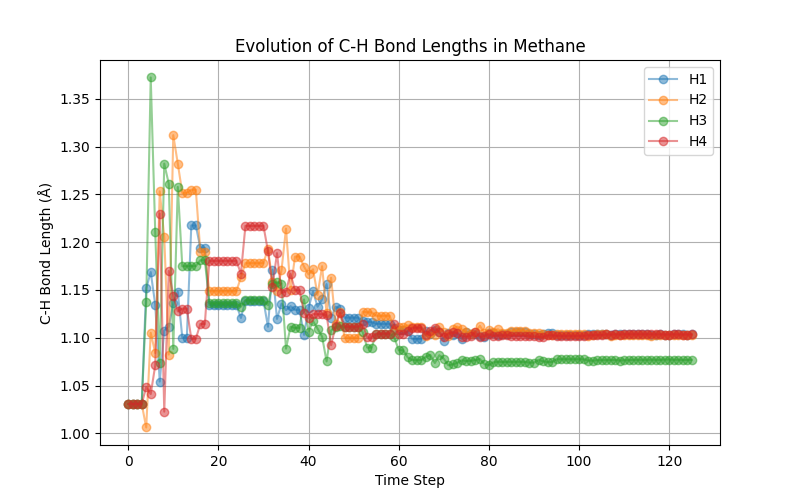
The above plot shows that we do not find the expected tetrahedral symmetry. The problem lies that our high-temperature dataset does not carry this information. We leave it as an exercise to the reader to retrain the potential using the low-temperature data and observe that one indeed recovers the expected tetrahedral shape.
Network utilization: geometry optimizaton of dihydrogen
The same neural network used for methane (CH₄) optimization can also be applied to the H₂ molecule. Although H₂ was not explicitly simulated during training, the dataset contains relevant atomic environments that provide some information about this system. By optimizing H₂ using the neural network, we can attempt to determine an optimal H-H bond distance. However, caution must be exercised when interpreting the resulting energy values, as the model was not explicitly trained for this specific molecular system. The predicted energy should be seen as an extrapolation rather than an exact value, and additional validation may be necessary to ensure meaningful results.
The following adjustments are made to the script:
import os
import time
import numpy as np
import ase.io
from ase import Atoms
from ase.visualize import view
from ase.data import atomic_numbers
import torch
from scipy.optimize import minimize
from perceptronium import SymmetryFunctionCalculator

# Define the root directory
ROOT = os.path.dirname(__file__)

def main():
    """
    Main function to optimize h2 molecule geometry using a trained neural network.
    """
    # Define atomic symbols and initial positions for H2
    symbols = ['H', 'H']
    positions = np.array([
        [-1.0, 0.0, 0.0],
        [ 1.0, 0.0, 0.0],
    ])

    # Create an ASE Atoms object (no periodic boundary conditions)
    h2 = Atoms(symbols=symbols, positions=positions)
    h2.center(vacuum = 0.0)

    # Initialize Symmetry Function Calculator
    sfc = SymmetryFunctionCalculator(os.path.join(ROOT, '..', 'data', 'request'),
                                    [atomic_numbers[element] for element in ['C', 'H']])

    # Load trained neural network model
    device = torch.device("cuda" if torch.cuda.is_available() else "cpu")
    torch.set_float32_matmul_precision('high')
    mask = torch.tensor(np.ones(len(h2))).to(device)
    model_path = os.path.join(ROOT, '..', 'output', 'ch4_network.pth')
    model = torch.load(model_path, weights_only=False)
    model.to(device).eval()
    model = torch.compile(model)

    # Track iteration history
    iteration_data = []  # Store energy and time per iteration
    position_data = []    # Store molecular positions per iteration
    start_time = time.time()  # Start timer
    bestenergy = float('inf')  # Initialize best energy as a large value
    energy = 0  # Initialize energy value

    def calculate_energy(pos):
        """
        Compute the energy of the system given atomic positions.
        """
        nonlocal energy

        # Compute symmetry function coefficients
        coeff = sfc.calculate(pos.reshape((len(h2), -1)), h2.get_atomic_numbers())
        input_tensor = torch.tensor(coeff, dtype=torch.float32).unsqueeze(0).to(device)

        # Perform inference with the trained model
        with torch.no_grad():
            energy = model(input_tensor, mask=mask).cpu().detach().numpy()[0, 0]
        return energy

    def callback(current_positions):
        """
        Callback function to track optimization progress.
        """
        nonlocal start_time, bestenergy, energy

        # Update best energy if improved
        if energy < bestenergy:
            bestenergy = energy
            position_data.append(current_positions.reshape((len(h2), -1)))

            # Compute elapsed time
            elapsed_time = time.time() - start_time
            start_time = time.time()  # Reset timer for next iteration

            # Store iteration data
            iteration_data.append((len(iteration_data) + 1, energy, elapsed_time))

            # Print iteration progress
            print(f"Iteration {len(iteration_data)}: Energy = {energy:.6f}, Time = {elapsed_time:.4f} sec")

    # Optimize molecular geometry using Nelder-Mead (Simplex Search)
    result = minimize(
        fun=calculate_energy,                       # Energy function
        x0=positions.flatten(),                     # Flattened initial positions
        method='Nelder-Mead',                       # Gradient-free optimization
        callback=callback,                          # Track iterations
        options={'maxiter': 5000, 'fatol': 1e-4}    # Stopping criteria
    )

    # Store optimized atomic configurations, add a unitcell mainly for
    # visualization purposes
    atoms_list = [Atoms(symbols=symbols, positions=pos) for pos in position_data]
    for atoms in atoms_list:
        atoms.set_cell([5.0, 5.0, 5.0])

        atoms.center()

    # store as animated gif
    ase.io.write(os.path.join(ROOT, '..', 'output', 'h2opt.gif'), atoms_list, format='gif', interval=100)

if __name__ == '__main__':
    main()
Optimization results for dihydrogen
The animated GIF illustrates the optimization process of an H₂ molecule, starting from an intentionally unfavorable bond distance. The script automatically adjusts the atomic positions by minimizing the predicted energy using a neural network model. However, since the dataset used to train the model does not explicitly include the optimal H₂ bond length, the predicted energy represents an extrapolation rather than an exact value. Despite this limitation, the final structure converges to a physically reasonable H–H distance, demonstrating the model’s ability to capture meaningful trends in atomic interactions.